4.1 Quick Review on Inference for Mean
4.1.1 Objectives
By the end of this unit, students will be able to:
- Distinguish between normal distribution and t distribution.
- Compute point estimates and confidence intervals for estimating one population mean based on one sample and paired samples.
4.1.2 Overview
In earlier discussions, we modeled the behavior of a sample proportion \(\hat{p}\) using the normal distribution, once certain conditions were satisfied. In this chapter, we extend those ideas to the sample mean \(\bar{x}\). The sampling distribution of \(\bar{x}\) also tends to follow a normal model when the sample is large and the data are independent. However, in most real-world applications, the population standard deviation \(\sigma\) is unknown. To account for this additional uncertainty, we replace \(\sigma\) with the sample standard deviation \(s\) and use a related family of distributions—the \(\textbf{t-distributions}\) —for inference about the mean.
The Sampling Distribution of \(\bar{x}\)
A sample mean computed from a random sample of size n has its own distribution, known as the sampling distribution of the sample mean. This distribution describes how \(\bar{x}\) varies from sample to sample.
Center: The mean of the sampling distribution equals the population mean (E(\(\bar{x}\))=\(\mu\)).
Spread: The standard deviation of this distribution, called the standard error (SE), measures the typical sampling fluctuation: SE_{\(\bar{x}\) } = \(\frac{\sigma}{\sqrt{n}}\) In practice, since \(\sigma\) is almost never known, we estimate it by using s, the sample standard deviation: SE_{\(\bar{x}\) } \(\approx \frac{s}{\sqrt{n}}\)
Shape: According to the Central Limit Theorem (CLT), when n is sufficiently large, the distribution of \(\bar{x}\) is approximately normal, even if the population itself is not.
Central Limit Theorem for the Sample Mean
When independent observations are drawn from a population with mean \(\mu\) and standard deviation \(\sigma\):
\[\bar{x} \sim N\!\left(\mu,\; \frac{\sigma}{\sqrt{n}}\right)\]
This powerful result allows us to make probability statements and construct confidence intervals for \(\mu\), even without observing the entire population.
Before we can apply the CLT, however, two major assumptions must hold:
- Independence — The observations in the sample must be independent. This is generally satisfied when data come from a simple random sample or a randomized experiment.
- Normality — For small samples, the population distribution should be approximately normal. For larger samples, this requirement becomes less strict.
Rules of Thumb for Assessing Normality
Because perfect normality is rare, we rely on pragmatic rules:
- When \(n<30\): As long as there are no strong outliers or heavy skew, the normal model is reasonable.
- When \(n\ge30\): The sampling distribution of \(\bar{x}\) is nearly normal, even for moderately skewed populations.
Intuition also helps: for highly skewed data—such as social-media follower counts—much larger samples are needed before the CLT approximation is reliable.
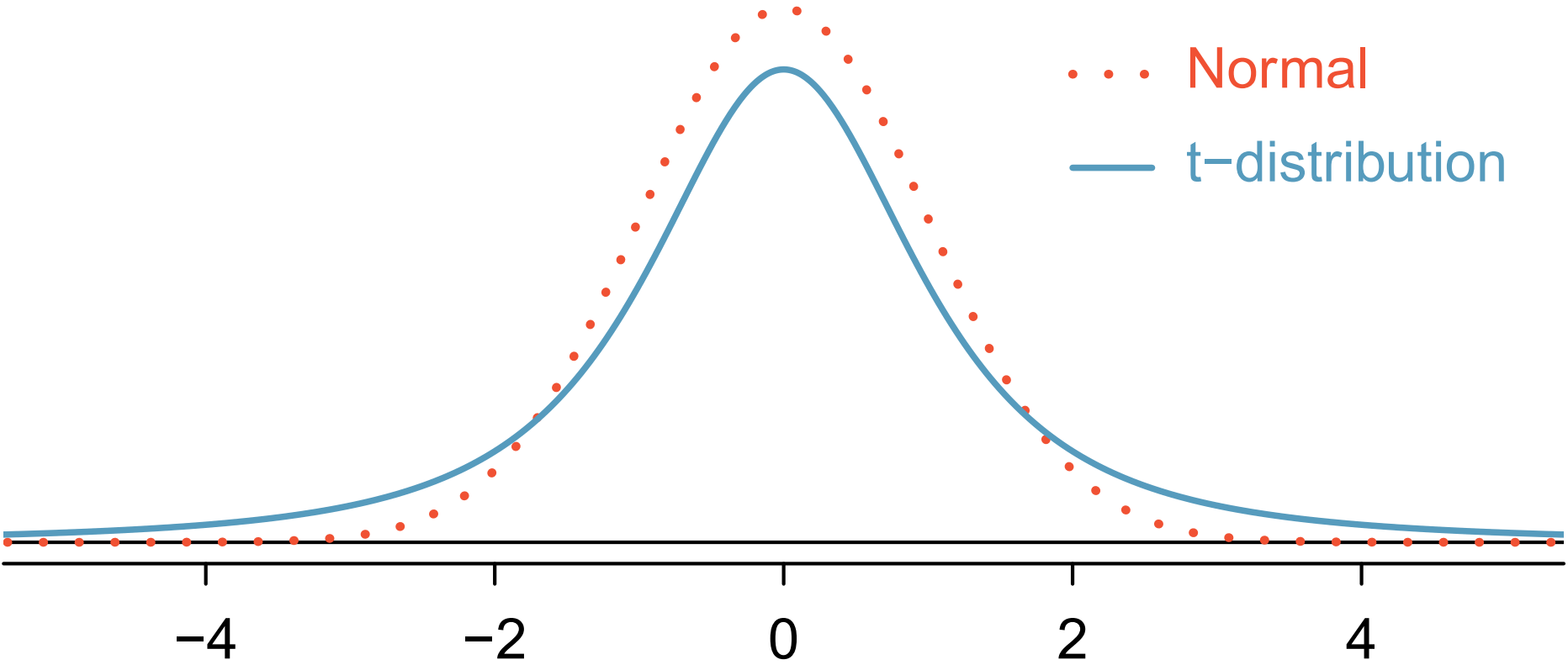
Introducing the t-Distribution
When we replace \(\sigma\) by the sample standard deviation s in the SE, the additional uncertainty causes the sampling distribution of \(\bar{x}\) to have thicker tails than the normal curve. This adjusted model is described by the t-distribution, which is centered at 0 and defined by a single parameter—the degrees of freedom (df):
\[df = n - 1\]
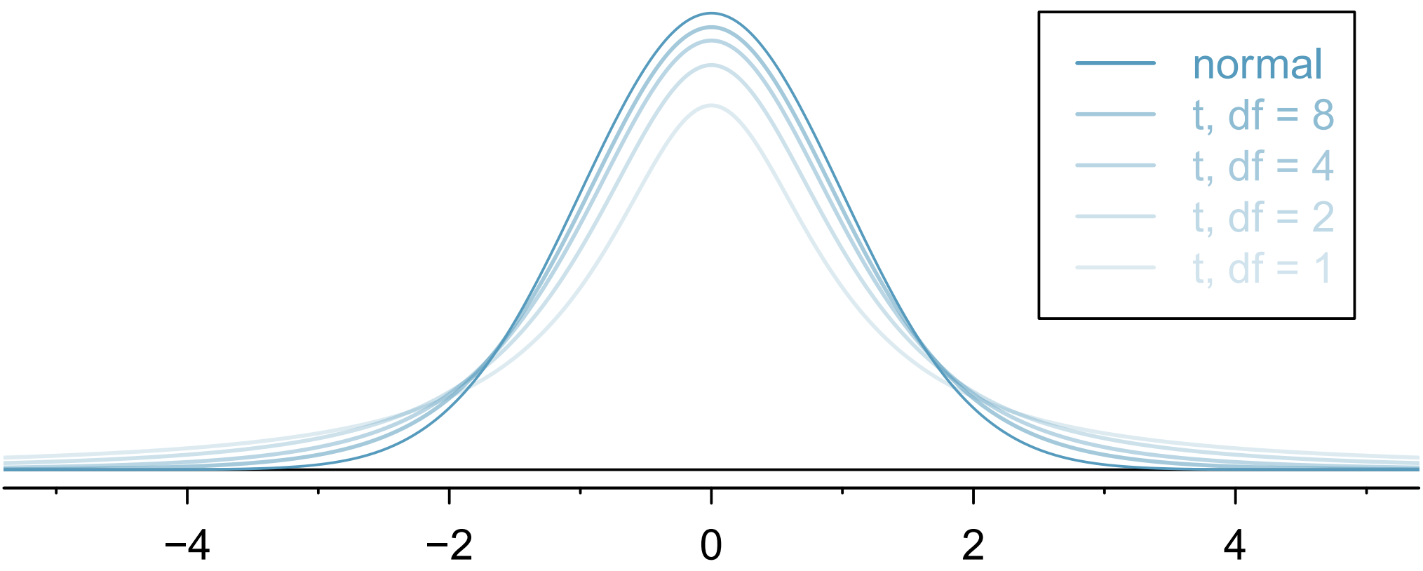
For small n, the t-distribution is wider (reflecting more uncertainty).
As n grows, the t-distribution becomes nearly identical to the normal distribution.
Thus, the t-distribution corrects for the extra variability introduced when using s instead of \(\sigma\) .

Confidence Intervals for a Single Mean
When the population standard deviation is unknown, a confidence interval for the population mean is constructed using the t-distribution:
\[\text{CI: } \bar{x} \pm t^*_{df} \times \frac{s}{\sqrt{n}}\]
where \(t^*_{df}\) is the critical value from the t-distribution with \(df=n-1\) corresponding to the desired confidence level (e.g., 90%, 95%, 99%).
Steps for Building a Confidence Interval:
Prepare: Identify the sample mean \(\bar{x}\) , standard deviation s, and sample size n.
Check Conditions: Confirm independence and approximate normality.
Calculate: Find the appropriate t^*_{df}, compute SE, and construct the interval.
Conclude: Interpret the result in context—for instance, “We are 95% confident that the true average completion time is between 92 and 96 minutes.”
One-Sample t-Tests
The hypothesis-testing procedure parallels the one for proportions but uses the t-distribution:
Define hypotheses:\(H_0: \mu = \mu_0 \ and \ H_A: \mu \ne \mu_0 (or >, <)\).
Compute the t-score: \[t = \frac{\bar{x} - \mu_0}{s / \sqrt{n}}\]
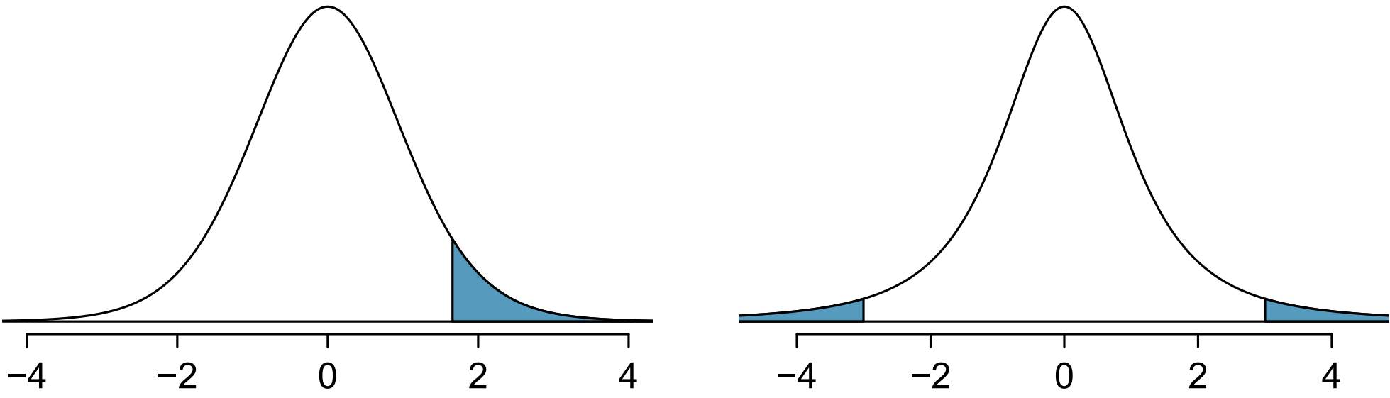
Determine the p-value by finding the tail area under the appropriate t-distribution.
Draw a conclusion based on the chosen significance level \(\alpha\).
Example:
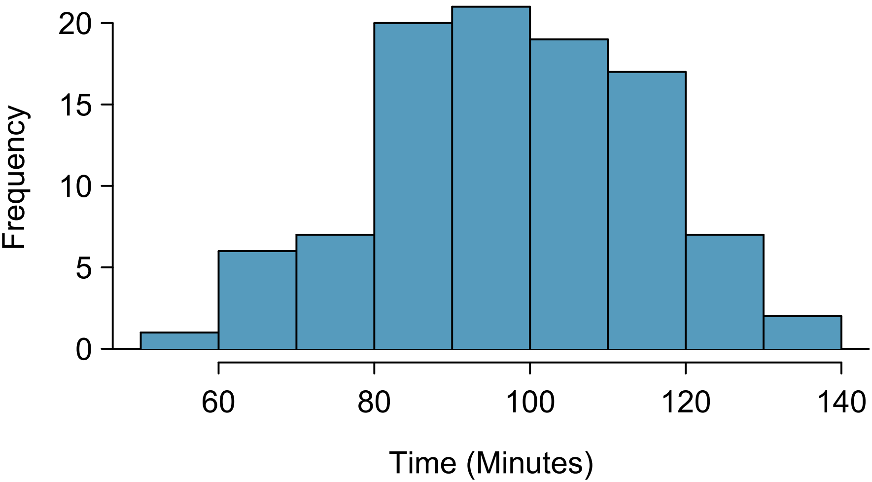
In the Cherry Blossom 10-mile Race, the mean finishing time in 2008 was 96.21 minutes. Using a random sample of 150 runners from 2018, we can test whether average times have changed. If independence and normality hold, the resulting p-value from the t-distribution indicates whether runners are significantly faster or slower today.
Distinguishing the Normal and t Distributions
Feature Normal Distribution t Distribution Shape Symmetrical bell curve Symmetrical but with thicker tails Spread Determined by known \(\sigma\) Depends on df (n-1); wider for small n Use When \(\sigma\) known or large sample \(\sigma\) unknown, small sample Approaches Normal? Always the same shape As \(df\) increases, \(t → Normal\)
To consider different degree of freedom:
Paired-Sample t-Intervals
When measurements are dependent—for example, “before and after” data for the same subjects—we analyze the differences:
\[d_i = X_{1i} - X_{2i}\]
The confidence interval for the mean difference is then:
\[\bar{d} \pm t^*_{df} \times \frac{s_d}{\sqrt{n}}\]
where \(\bar{d}\) and s_d are the mean and standard deviation of the differences. This method isolates the treatment effect by removing variability between subjects.
Summary - A point estimate (such as \(\bar{x}\) ) provides a single best guess for \(\mu\), but it is subject to sampling error.
The Central Limit Theorem ensures that \(\bar{x}\) is approximately normal for large, independent samples.
When \(\sigma\) is unknown, we use the t-distribution, which adjusts for additional uncertainty.
Confidence intervals combine estimation and uncertainty into one statement: \(\text{Estimate} \pm t^* \times SE\).
One-sample and paired-sample t-tests extend these ideas to formal hypothesis testing.
Together, these tools allow us to move from descriptive summaries to inferential conclusions about population means—building the bridge between data and decision-making.
4.1.4 Solved Exercises
Exercise 1
Find the probability that a t-distributed random variable with 10 degrees of freedom is less than 1.25.
\[ P(T < 1.25) \]
Solution:
Exercise 2
Find the probability that a t-distributed random variable with 12 degrees of freedom is greater than 2.18.
\[ P(T > 2.18) \]
Solution:
Exercise 3
Find the probability that a t-distributed random variable with 15 degrees of freedom lies between -1.25 and 1.25.
\[ P(-1.25 < T < 1.25) \]
Solution:
Exercise 4
Find the critical t-value, \(t_{\alpha/2}\), for a 95% confidence level with 20 degrees of freedom.
Solution:
Exercise 5
Construct a 90% confidence interval for a sample with:
\[ n = 9, \quad \bar{x} = 50.2, \quad s = 4.8 \]
Step 1: Find \(t_{\alpha/2}\) for \(df = n - 1 = 8\) and \(CL = 90\%\)
Step 2: Compute the Standard Error
\[ SE = \frac{s}{\sqrt{n}} = \frac{4.8}{\sqrt{9}} = 1.6 \]
Step 3: Compute the Margin of Error
\[ ME = t^* \times SE = 1.8595 \times 1.6 = 2.975 \]
Step 4: Construct the Confidence Interval
\[ \bar{x} \pm ME = 50.2 \pm 2.975 = (47.225,\ 53.175) \]
Solution:
The 90% confidence interval for the mean is:
\[ (47.23,\ 53.18) \]