4.2 Hypothesis Testing for mean \(\mu\)
4.2.1 Objectives
By the end of this unit, students will be able to:
- Formulate claims about a population mean in the form of a null hypothesis and alternative hypothesis.
- Conduct t-tests for testing claims about a single population mean based on one sample and paired samples.
4.2.2 Overview
Inference for a mean follows the same high-level path as inference for a proportion: state hypotheses, compute a standardized statistic, obtain a p-value from a reference distribution, and compare to a pre-specified significance level \(\alpha\). Because the population standard deviation \(\sigma\) is rarely known, we estimate it with the sample standard deviation s and use the \(\textbf{t distribution}\) with \(df=n-1\). This choice reflects the extra uncertainty from substituting s for \(\sigma\).
One-Sample t-Test:
When to Use the one sample t-Test is listed below when:
You have a single random sample of quantitative data.
You want to test a claim about the population mean \(\mu\).
Conditions for use:
Independence: observations arise from a simple random sample, random assignment, or sampling less than 10% of the population.
Normality: for small n, data should be roughly symmetric with no extreme outliers; for n \(\ge\) 30, the t-test is robust to moderate skew.
Steps in Hypothesis Testing
- State the Hypotheses
\[H_0: \mu = \mu_0 \qquad \text{vs.} \qquad H_A: \mu \ne \mu_0\]
Compute the Test Statistic
Using sample size n, mean \(\bar{x}\), and standard deviation s:
\[T = \frac{\bar{x} - \mu_0}{s / \sqrt{n}}, \qquad df = n - 1\]
Find the p-value
The p-value represents the probability of obtaining a result as extreme or more extreme than the observed one, assuming H_0 is true.
Use R functions:
Left-tailed: pt(t, df)
Right-tailed: pt(t, df, lower.tail = FALSE)
Two-tailed: 2 * pt(-abs(t), df)
Make a Decision Compare the p-value to the significance level \(\alpha\) (commonly 0.05):
If \(p \le \alpha\): reject H_0 → sufficient evidence for H_A.
If \(p > \alpha\): fail to reject H_0 → insufficient evidence for H_A.
Paired-Sample t-Test
Paired designs arise when each subject (or matched unit) provides two related measurements — for instance, before and after treatment. We compute the difference for each pair:
\[d_i = X_{1i} - X_{2i}, \qquad i = 1, 2, \ldots, n\]
Then analyze these differences as a single sample.
Hypotheses
\[H_0: \mu_d = 0 \qquad \text{vs.} \qquad H_A: \mu_d \ne 0\]
Test Statistic
\[T = \frac{\bar{d} - 0}{s_d / \sqrt{n}}, \qquad df = n - 1\]
Example: Trader Joe’s vs. Safeway Grocery Prices
In a previous local study, researchers found that Trader Joe’s prices were, on average, lower than those at Safeway for similar grocery items in 2015. Nearly a decade later, both stores have adjusted to inflation and competition from online retailers. We wondered: How do the prices compare today?
We sampled 68 common grocery items sold at both Trader Joe’s and Safeway. A portion of the dataset is shown below, with prices in U.S. dollars.
| item_number | item_name | safeway | trader_joes | price_difference |
|---|---|---|---|---|
| 1 | Organic milk (1 gal) | 5.29 | 4.99 | 0.30 |
| 2 | Brown eggs (dozen) | 4.19 | 3.79 | 0.40 |
| 3 | Peanut butter (16 oz) | 3.99 | 3.49 | 0.50 |
| … | … | … | … | … |
| 68 | Greek yogurt (pack 4) | 6.59 | 5.99 | 0.60 |
We define the paired difference as:
\[\text{Difference} = \text{Safeway Price} - \text{Trader Joe's Price}\]
Positive differences indicate that Safeway is more expensive. A histogram of the price differences is shown below:
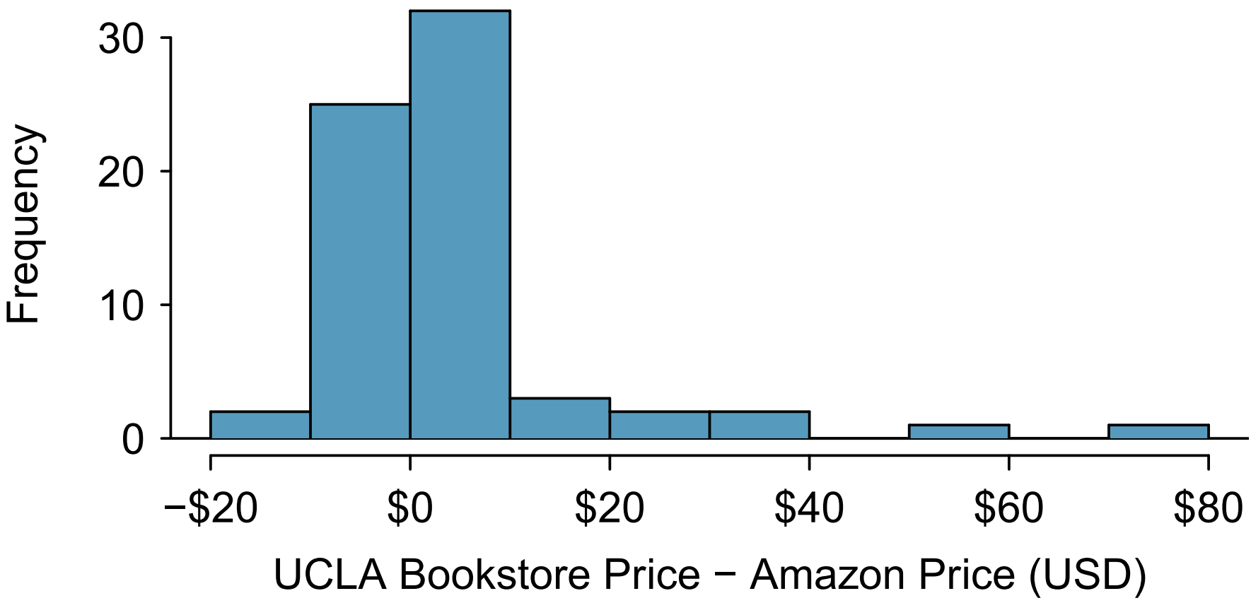
Sample statistics:
\[n_{diff} = 68, \quad \bar{x}_{diff} = 0.58, \quad s_{diff} = 1.79\]
We test whether the average price difference is zero:
\[H_0: \mu_{diff} = 0 \quad \text{vs.} \quad H_A: \mu_{diff} \ne 0\]
Compute the standard error and test statistic:
\[ SE_{\bar{x}{diff}} = \frac{s{diff}}{\sqrt{n_{diff}}} = \frac{1.79}{\sqrt{68}} = 0.217\\ T = \frac{\bar{x}{diff} - 0}{SE{\bar{x}_{diff}}} = \frac{0.58}{0.217} = 2.67, df = 67 \]
The two-tailed p-value corresponds to the shaded tails in the \(t_{67}\) distribution below
## [1] 0.009509096Paired Confidence Interval
The \((1 - \alpha)100%\) confidence interval for the mean difference is:
\[\bar{d} \pm t^*_{df} \frac{s_d}{\sqrt{n}}\]
n <- 68
dbar <- 0.58
sd_d <- 1.79
df <- n - 1
se_d <- sd_d / sqrt(n)
conf <- 0.95
t_star <- qt(1 - (1 - conf)/2, df = df)
ci <- c(dbar - t_star*se_d, dbar + t_star*se_d)
ci
## [1] 0.1467277 1.0132723Interpretation: We are 95% confident that the average difference in prices (Bookstore - Amazon) falls within this interval. Since the interval is entirely above 0, bookstore prices tend to be higher.
Practical Guidelines:
Verify conditions: Independence and approximate normality (of raw data or paired differences). For \(n \ge 30\), the t-procedure is generally robust to mild skewness.
Predefine direction: Choose between two-sided and one-sided tests before analyzing data.
Report clearly: Always present t, df, p, and the contextual interpretation, plus a CI for effect size.
4.2.4 Solved Exercises
Exercise 1
Without finding the values, arrange the numbers from small to large:
- \(P(Z < -1.40)\)
- \(P(T < -1.40)\) with \(df=9\)
- \(P(T < -1.40)\) with \(df=14\)
- \(P(Z > 1.20)\)
- \(P(T > 1.20)\) with \(df=9\)
- \(P(T > 1.20)\) with \(df=14\)
\[ \_\_\_\_\_\_ < \_\_\_\_\_\_ < \_\_\_\_\_\_ < \_\_\_\_\_\_ < \_\_\_\_\_\_ < \_\_\_\_\_\_ \]
Solution
Recall that the t-distribution has heavier tails than the z-distribution, so probabilities farther from the mean will be larger for t. Also, as the degrees of freedom increase, t becomes closer to z.
Smallest to largest:
\[P(Z < -1.40) < P(T < -1.40, df=14) < P(T < -1.40, df=9) < P(Z > 1.20) < P(T > 1.20, df=14) < P(T > 1.20, df=9)\]
Exercise 2
Use R calculator to find the values of the probability of t-distribution. Sketch the t-curve and shaded region.
- \(P(T < -1.40)\) with \(df=9\)
- \(P(T < -1.40)\) with \(df=14\)
- \(P(T > 1.20)\) with \(df=9\)
- \(P(T > 1.20)\) with \(df=14\)
Solution
pt(-1.40, df=9)     # 0.0948
pt(-1.40, df=14)    # 0.0905
pt(1.20, df=9, lower.tail=FALSE)  # 0.1266
pt(1.20, df=14, lower.tail=FALSE) # 0.1233
Exercise 3
Use R calculator to find the critical t-value \((t_{\alpha/2})\), rounding to 4 decimal places.
- CL = 90%, \(n = 9\)
- CL = 98%, \(n = 22\)
- CL = 99%, \(n = 30\)
- CL = 95%, \(n = 11\)
Solution
Degrees of freedom \(df = n - 1\).
qt(0.95, df=8)   # 1.8595
qt(0.99, df=21)  # 2.5176
qt(0.995, df=29) # 2.7564
qt(0.975, df=10) # 2.2281| Confidence Level | df | \(\alpha/2\) | \(t_{\alpha/2}\) |
|---|---|---|---|
| 90% | 8 | 0.05 | 1.8595 |
| 98% | 21 | 0.01 | 2.5176 |
| 99% | 29 | 0.005 | 2.7564 |
| 95% | 10 | 0.025 | 2.2281 |
Exercise 4
Find confidence intervals using the following sample information:
- \(n=6, \bar{x}=5.3, s=1.5\), 90% confidence level
- \(n=18, \bar{x}=5.3, s=1.5\), 90% confidence level
- \(n=6, \bar{x}=5.3, s=1.5\), 98% confidence level
- \(n=18, \bar{x}=5.3, s=1.5\), 98% confidence level
# (a)
t_a <- qt(0.95, df=5); ME_a <- t_a * 1.5/sqrt(6)
c(5.3 - ME_a, 5.3 + ME_a)

# (b)
t_b <- qt(0.95, df=17); ME_b <- t_b * 1.5/sqrt(18)
c(5.3 - ME_b, 5.3 + ME_b)

# (c)
t_c <- qt(0.99, df=5); ME_c <- t_c * 1.5/sqrt(6)
c(5.3 - ME_c, 5.3 + ME_c)

# (d)
t_d <- qt(0.99, df=17); ME_d <- t_d * 1.5/sqrt(18)
c(5.3 - ME_d, 5.3 + ME_d)| Case | df | CL | \(t_{\alpha/2}\) | Margin of Error | Confidence Interval |
|---|---|---|---|---|---|
| (a) | 5 | 90% | 2.015 | 1.23 | (4.07, 6.53) |
| (b) | 17 | 90% | 1.740 | 0.62 | (4.68, 5.92) |
| (c) | 5 | 98% | 3.365 | 2.06 | (3.24, 7.36) |
| (d) | 17 | 98% | 2.567 | 0.91 | (4.39, 6.21) |
Exercise 5
What factors influence the width of a confidence interval?
Solution:
Confidence level: Higher confidence \(\Rightarrow\) wider interval.
Sample size (n): Larger \(n \Rightarrow\) smaller standard error \(\Rightarrow\) narrower interval.
Sample variability (s): Larger \(s \Rightarrow\) wider interval.
From Exercise 4, increasing \(n\) narrows the interval, while increasing the confidence level widens it.
Exercise 6
A 95% confidence interval for \(\mu\) is given as (22.50, 23.70) based on a sample of 49.
Find: (a) \(\bar{x}\) (b) Margin of error (c) \(t_{\alpha/2}\) (d) Standard error (e) Sample SD
mean <- (22.50 + 23.70)/2        # 23.10
ME <- (23.70 - 22.50)/2          # 0.60
t <- qt(0.975, df=48)            # 2.010
SE <- ME / t                     # 0.2985
s <- SE * sqrt(49)               # 2.09
mean; ME; t; SE; s
Exercise 7
Find the P-value for the given sample sizes and test statistics:
- \(n=24\), \(T=2.315\), right-tailed
- \(n=16\), \(T=-1.60\), left-tailed
- \(n=24\), \(T=2.315\), two-tailed
- \(n=16\), \(T=-1.60\), two-tailed
# a
1 - pt(2.315, df=23)     # 0.0159
# b
pt(-1.60, df=15)         # 0.0653
# c
2*(1 - pt(2.315, df=23)) # 0.0318
# d
2*pt(-1.60, df=15) # 0.1306| Case | Tail | P-value | Decision (\(\alpha=0.05\)) |
|---|---|---|---|
| (a) | Right | 0.0159 | Reject \(H_0\) |
| (b) | Left | 0.0653 | Fail to reject \(H_0\) |
| (c) | Two | 0.0318 | Reject \(H_0\) |
| (d) | Two | 0.1306 | Fail to reject \(H_0\) |
Exercise 8
A random sample of 25 Seattle residents reported their daily coffee intake:
\[ n = 25, \quad \bar{x} = 2.7, \quad s = 0.9 \]
A nutritionist claims that Seattle residents drink more than 2 cups per day on average.
Is the result statistically significant?
Follow the steps to conduct the hypothesis test.
- Write the hypotheses
\[ H_0: \mu = 2 \\ H_a: \mu > 2 \]
- Calculate the test statistic
\[ T = \frac{\bar{x} - \mu_0}{s / \sqrt{n}} = \frac{2.7 - 2}{0.9 / \sqrt{25}} = \frac{0.7}{0.18} = 3.89 \]
(c) Compute the P-value and draw a picture
- Conclusion (using \(\alpha = 0.05\))
Since \(P < 0.05\), we reject \(H_0\). There is strong evidence that Seattle residents drink more than 2 cups of coffee per day on average.
- Confidence interval interpretation
A 90% confidence interval corresponding to this hypothesis test would not include 2, which supports the conclusion from the hypothesis test.