5.1 Introduction to Linear Regression
5.1.1 Objectives
By the end of this unit, students will be able to:
- Describe linear associations between numerical variables using correlations.
- Use linear regression to model linear relationships between two numerical variables.
- Evaluate the statistical significance of linear relationships between numerical variables.
5.1.2 Overview
Regression analysis concerns the study of relationships between quantitative variables—identifying, estimating, and validating those relationships.
Simple linear regression explores whether the relationship between two numerical variables is linear and quantifies the strength and direction of the association.
We begin with a scatter plot of two numerical variables to assess whether a linear pattern is present.
If the data suggest a linear relationship, we use the linear model \(y = \beta_0 + \beta_1x\) to best describe the relationship between the variables.
From a random sample of paired observations \((x_i, y_i)\) for \(i = 1, \ldots, n\) we estimate this relationship using the least-squares method, yielding the fitted model \(\hat{y} = b_0 + b_1x\).
Simple linear regression uses a single numerical predictor to forecast a numerical response. The model assumes a straight-line form:
\[\displaystyle{y = \beta_0 + \beta_1x + \varepsilon}\]
where \(\beta_0\) is the intercept, \(\beta_1\) is the slope, and \(\varepsilon\) random error term representing unexplained variation. We often assume that \(\varepsilon \sim N(0, \sigma)\), meaning the errors follow a normal distribution with mean 0 and constant variance \(\sigma^2\). The expected value of y at any given x is:
\[\displaystyle{\mathbb{E}\left[y\right] = \beta_0 + \beta_1x}\]
Let’s see regression in action as we consider an application to understanding biases in course evaluations.
Understanding Bias in Course Evaluations:
Many colleges collect student evaluations at the end of each course. However, researchers have debated whether these ratings truly reflect teaching effectiveness or if they are influenced by unrelated factors, such as the instructor’s appearance. Hamermesh and Parker (2005) found that instructors perceived as more attractive tended to receive higher teaching evaluations.(Daniel S. Hamermesh, Amy Parker, Beauty in the classroom: instructors pulchritude and putative pedagogical productivity, Economics of Education Review, Volume 24, Issue 4, August 2005, Pages 369-376, ISSN 0272-7757, 10.1016/j.econedurev.2004.07.013. http://www.sciencedirect.com/science/article/pii/S0272775704001165.)
In this section, we will examine data adapted from that study to explore whether beauty ratings are correlated with course evaluation scores.
| variable | description |
|---|---|
score |
average professor evaluation score: (1) very unsatisfactory - (5) excellent. |
rank |
rank of professor: teaching, tenure track, tenured. |
ethnicity |
ethnicity of professor: not minority, minority. |
gender |
gender of professor: female, male. |
language |
language of school where professor received education: english or non-english. |
age |
age of professor. |
cls_perc_eval |
percent of students in class who completed evaluation. |
cls_did_eval |
number of students in class who completed evaluation. |
cls_students |
total number of students in class. |
cls_level |
class level: lower, upper. |
cls_profs |
number of professors teaching sections in course in sample: single, multiple. |
cls_credits |
number of credits of class: one credit (lab, PE, etc.), multi credit. |
bty_f1lower |
beauty rating of professor from lower level female: (1) lowest - (10) highest. |
bty_f1upper |
beauty rating of professor from upper level female: (1) lowest - (10) highest. |
bty_f2upper |
beauty rating of professor from second upper level female: (1) lowest - (10) highest. |
bty_m1lower |
beauty rating of professor from lower level male: (1) lowest - (10) highest. |
bty_m1upper |
beauty rating of professor from upper level male: (1) lowest - (10) highest. |
bty_m2upper |
beauty rating of professor from second upper level male: (1) lowest - (10) highest. |
bty_avg |
average beauty rating of professor. |
pic_outfit |
outfit of professor in picture: not formal, formal. |
pic_color |
color of professor’s picture: color, black & white. |
Prediction (Predicted value)
If the least-squares regression line is given by \(\hat{y} = b_0 + b_1x\), then for a particular value of x, the predicted value is simply \(\hat{y} = b_0 + b_1x\).
- The slope \(b_1\) represents the average change in the predicted response y for each additional unit of \(x\).
- The intercept b_0 represents the predicted value of \(y\) when \(x = 0\).
Residual
For each observation i, \(e_i = y_i - \hat{y}_i = y_i - (b_0 + b_1x_i)\) represents the prediction error or residual. Residual plots help verify linearity and check whether variability remains roughly constant.
The Correlation Coefficient
The correlation coefficient measures the strength and direction of a linear association:
\(R = \frac{1}{n-1}\sum_{i=1}^n \frac{(x_i - \bar{x})(y_i - \bar{y})}{s_x s_y}\)
with \(R\): \(-1 \leq R \leq 1\). The closer \(|R|\) is to 1, the stronger the linear association.
The coefficient of determination, \(R^2\), represents the proportion of variability in the response variable that can be explained by the predictor:
\[R^2 = \frac{\text{Explained Variation}}{\text{Total Variation}}\]
Conditions to have the least squares regression
Visually inspect the scatter plot:
- The relationship between the explanatory and the response variable should be linear.
- The histogram of residuals distribution should be normal (symmetric, bell-shaped).
- The variability of points should be roughly constant.
- No extreme outliers.
Computing the coefficients in \(\hat{y} = b_0 + b_1x\)
\(b_1 = \frac{s_y}{s_x} R\)
\(b_0 = \bar{y} - b_1 \bar{x}\)
Hypothesis Testing for the Regression Slope
To determine whether the observed linear relationship is statistically significant, we test:
\(H_0: \beta_1 = 0 \quad \text{(no linear relationship)}\)
\(H_A: \beta_1 \ne 0 \quad \text{(a linear relationship exists)}\)
The test statistic is
\[t = \frac{b_1 - 0}{SE_{b_1}}, \qquad df = n - 2\]
where
\[SE_{b_1} = \frac{s}{\sqrt{\sum (x_i - \bar{x})^2}} \quad \text{and} \quad s = \sqrt{\frac{\sum e_i^2}{n-2}}.\]
If the p-value is less than the significance level \(\alpha = 0.05\), we reject \(H_0\) and conclude that a significant linear relationship exists.
Confidence Interval for the Slope
A \(100(1-\alpha)\%\) confidence interval for the true slope \(\beta_1\) is given by:
\[b_1 \pm t^*{df} \times SE{b_1}\]
Interpretation:
“We are 95% confident that the average change in y for every one-unit increase in \(x\) lies between the lower and upper bounds of this interval.”
Example: Relationship Between Study Hours and Exam Scores at North Carolina A&T State University
At North Carolina A&T State University (NCAT), an instructor wants to explore whether the number of hours students spend studying per week is related to their exam performance. Each observation represents a randomly selected NCAT student enrolled in an introductory statistics course. Is there a significant linear relationship between hours studied and exam score among NCAT students?
set.seed(2025)
hours_studied <- sample(1:15, 20, replace = TRUE)
exam_score <- round(50 + 3 * hours_studied + rnorm(20, mean = 0, sd = 5), 1)

ncat_data <- data.frame(hours_studied, exam_score)
head(ncat_data)
The dataset represents students from North Carolina A&T State University, showing the number of hours each student studied during the week and their corresponding exam scores; study hours range from 1 to 14, and exam scores range from 51.8 to 101.10, providing information to explore whether the amount of study time is related to exam performance.
We then fit the model as follows:
##
## Call:
## lm(formula = exam_score ~ hours_studied, data = ncat_data)
##
## Residuals:
##    Min     1Q Median     3Q    Max
## -8.940 -3.173 -1.075  3.314 12.905
##
## Coefficients:
##               Estimate Std. Error t value Pr(>|t|)
## (Intercept)    52.0230     3.2334  16.089 3.97e-12 ***
## hours_studied   2.8431     0.3377   8.418 1.18e-07 ***
## ---
## Signif. codes:  0 '***' 0.001 '**' 0.01 '*' 0.05 '.' 0.1 ' ' 1
##
## Residual standard error: 5.867 on 18 degrees of freedom
## Multiple R-squared:  0.7974, Adjusted R-squared:  0.7862
## F-statistic: 70.86 on 1 and 18 DF,  p-value: 1.178e-07
The intercept (52.02) suggests that if a student does not study at all, their predicted exam score would be about 52 points. The slope (2.84) indicates that for each additional hour studied, the predicted exam score increases by approximately 2.84 points on average. This shows a positive relationship between study time and exam performance, as students spend more hours studying, their exam scores tend to increase. The p-value for hours studied (1.18e-07) is far less than 0.05, meaning the relationship is highly statistically significant. The R-squared value (0.797) indicates that about 79.7% of the variation in exam scores can be explained by the number of study hours, suggesting the model provides a very good fit to the data. The F-statistic (70.86, p < 0.001) further confirms that the overall regression model is statistically significant. The p-value for the slope (0.043) is less than 0.05, meaning the relationship is statistically significant at the 5% level.
5.1.4 Solved Exercises
Exercise 1
Describe the linear relationship from the scatter plot.
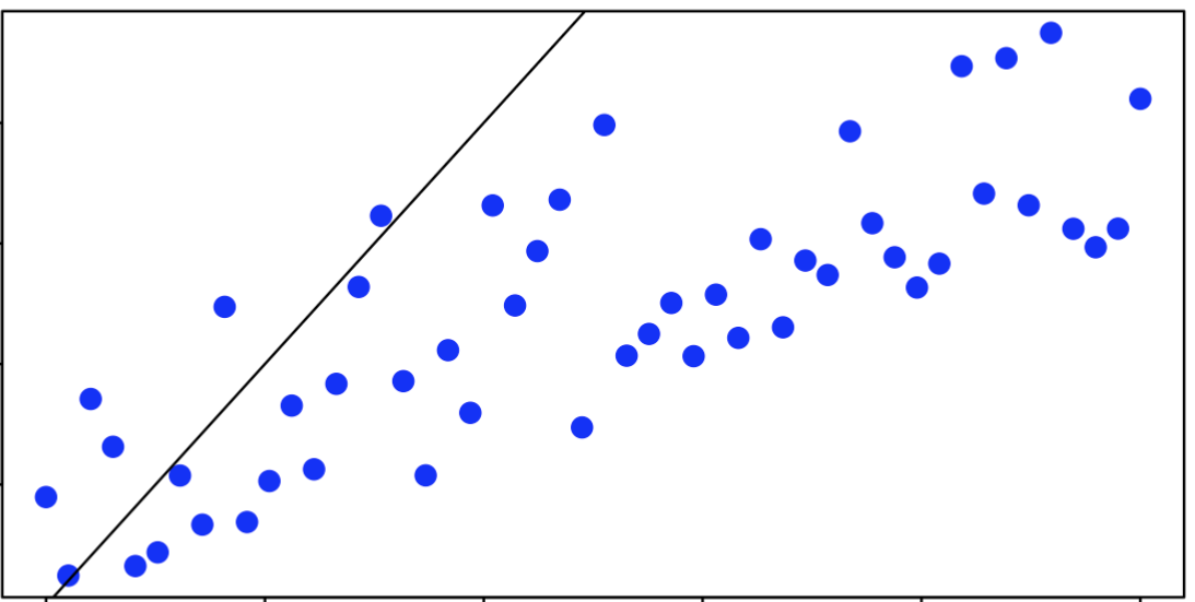
Select the correct choice.
(a) Strong positive relationship
(b) Strong negative relationship
(c) Weak positive relationship
(d) Weak negative relationship
Solution: (c) Weak positive relationship
Exercise 2
The mean travel time from one stop to the next on the Rocky Mountain Express train is 142 minutes, with a standard deviation of 120 minutes. The mean distance from one stop to the next is 115 miles, with a standard deviation of 100 miles. The correlation between travel time and distance is 0.612.
(a) Write the equation of the regression line for predicting travel time based on distance.
Solution (a):
The regression slope is calculated as:
\[ b_1 = r \frac{s_y}{s_x} = 0.612 \times \frac{120}{100} = 0.7344 \]
The intercept is:
\[ b_0 = \bar{y} - b_1 \bar{x} = 142 - 0.7344 \times 115 = 142 - 84.456 = 57.544 \]
So the regression equation is:
\[ \hat{y} = 57.544 + 0.7344 x \]
(b) Interpret the slope and intercept.
Solution (b):
- Slope (\(b_1 = 0.7344\)): For every additional mile between stops, the predicted travel time increases by approximately 0.73 minutes.
- Intercept (\(b_0 = 57.544\)): If the distance between stops were 0 miles, the predicted travel time would be approximately 57.5 minutes (theoretically).
(c) Calculate and interpret \(R^2\).
Solution (c):
\[ R^2 = r^2 = (0.612)^2 = 0.3745 \approx 37.5\% \]
Interpretation: About 37.5% of the variation in travel time can be explained by the distance between stops.
(d) The distance between Denver and Boulder is 110 miles. Use this model to estimate the travel time.
Solution (d):
\[ \hat{y} = 57.544 + 0.7344 \times 110 = 57.544 + 80.784 = 138.328 \text{ minutes} \]
Predicted travel time: approximately 138.3 minutes.
(e) It actually takes 165 minutes. Calculate the residual. Is the model overestimating or underestimating?
Solution (e):
Residual:
\[ e = y_{\text{observed}} - \hat{y} = 165 - 138.328 = 26.672 \text{ minutes} \]
The residual is positive, so the model underestimates the actual travel time.
Example 2 Continued Below is an example of using the lm() function to perform a linear regression. Here, we define time using the regression equation obtained above for demonstration purposes. In real situations, however, the true regression equation is unknown — we use lm() to estimate it from data.
An example of how to interpret the resulting output is shown below:
# Example data (for demonstration)
distance <- c(80, 100, 120, 140, 160, 180, 200)
time <- 57.544 + 0.7344 * distance + rnorm(7, 0, 10)

# Fit regression model
model <- lm(time ~ distance)

# View summary output
summary(model)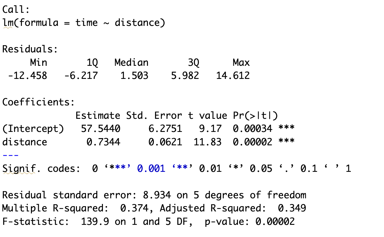
| Question | Where to Find It | Answer |
|---|---|---|
| (a) Regression Equation | Coefficients table | \(\hat{y}\) = 57.544 + 0.7344 × distance |
| (b) Interpret slope | Slope under distance |
For every additional mile, travel time ↑ by 0.734 minutes |
| (b) Interpret intercept | Intercept row | When distance = 0, predicted time \(\approx\) 57.5 min |
| (c) ( \(R^2\) ) | “Multiple R-squared” | ( R^2 = 0.374 ), i.e., 37.4% of variance explained |
| (d) Prediction | Use equation | ( \(\hat{y}\) = 57.544 + 0.7344(110) = 138.33 ) minutes |
| (e) Residual | Compare observed and predicted | ( e = 165 - 138.33 = +26.67 ); model underestimates |