3.2 Confidence Interval
3.2.1 Objectives
- Understand the meaning of sampling distributions.
- Apply the central limit theorem to define the sampling distribution of a sample proportion.
- Identify the conditions needed for the central limit theorem to apply for sample proportions.
- Construct and interpret confidence intervals for the population proportion.
3.2.2 Overview
1. Concept of Confidence Intervals
A point estimate (like \(\hat{p}\)) provides a single best guess of a population parameter. However, because samples vary, a single estimate rarely captures the true parameter value exactly.
To improve our estimation, we report a range of plausible values — called a confidence interval (CI) — that is likely to contain the population parameter.
A confidence interval therefore reflects two components:
- the point estimate (center), and
- the margin of error (distance from the estimate to each bound of the interval).
Definition
A confidence interval gives a plausible range of values for a population parameter such that, in repeated random samples, a specified proportion (confidence level) of these intervals will capture the true parameter.
Common confidence levels are 90%, 95%, and 99%.
A 95% confidence interval means that if we were to repeatedly take random samples of the same size and construct confidence intervals for each, approximately 95% of those intervals would contain the true population proportion \(p\).
Formula for a Confidence Interval for a Proportion
From the Central Limit Theorem, when sample size is sufficiently large and independence is satisfied,
the sampling distribution of \(\hat{p}\) is approximately normal:
\[ \hat{p} \sim N\left(p, \sqrt{\frac{p(1-p)}{n}}\right) \]
When \(p\) is unknown, we use \(\hat{p}\) in its place to estimate the standard error:
\[ S.E._{\hat{p}} = \sqrt{\frac{\hat{p}(1-\hat{p})}{n}} \]
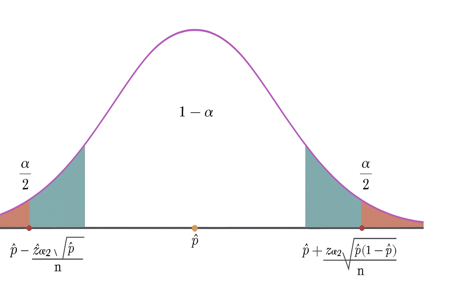
Hence, the \((1-\alpha)100\%\) confidence interval for the population proportion is:
\[ \boxed{\hat{p} \pm z_{\alpha/2}\sqrt{\frac{\hat{p}(1-\hat{p})}{n}}} \]
where:
- \(\hat{p}\) = sample proportion,
- \(z_{\alpha/2}\) = critical value from the standard normal distribution corresponding to the desired confidence level,
- \(n\) = sample size.
—
Critical Value \(z_{\alpha/2}\)
The critical value \(z_{\alpha/2}\) marks the cutoff points on the standard normal curve that capture the central \((1-\alpha)\) proportion of the distribution.
3.2.4 Solved Exercises
Exercise 1
Construct a 95% confidence interval using a sample proportion \(\hat{p} = 0.42\) and sample size \(n = 1200\).
Construct a 90% confidence interval using a sample proportion \(\hat{p} = 0.42\) and sample size \(n = 1200\).
Construct a 95% confidence interval using a sample proportion \(\hat{p} = 0.42\) and sample size \(n = 150\).
Solution:
The general formula for a confidence interval for a population proportion is:
\[ \hat{p} \pm z_{\alpha/2} \sqrt{\frac{\hat{p}(1-\hat{p})}{n}} \]
# Exercise 1 calculations
p_hat <- 0.42

# (a) 95% CI, n = 1200
n1 <- 1200
z_95 <- 1.96
SE1 <- sqrt(p_hat * (1 - p_hat) / n1)
ME1 <- z_95 * SE1
CI1 <- c(p_hat - ME1, p_hat + ME1)

# (b) 90% CI, n = 1200
z_90 <- 1.645
ME2 <- z_90 * SE1
CI2 <- c(p_hat - ME2, p_hat + ME2)

# (c) 95% CI, n = 150
n3 <- 150
SE3 <- sqrt(p_hat * (1 - p_hat) / n3)
ME3 <- z_95 * SE3
CI3 <- c(p_hat - ME3, p_hat + ME3)

list(CI_95_n1200 = CI1, CI_90_n1200 = CI2, CI_95_n150 = CI3)
## $CI_95_n1200
## [1] 0.3920743 0.4479257
##
## $CI_90_n1200
## [1] 0.3965624 0.4434376
##
## $CI_95_n150
## [1] 0.3410142 0.4989858Exercise 2
Circle the proper choices.
(a) The confidence interval is (wider/narrower) if the sample size increases.
(b) The confidence interval is (wider/narrower) if the confidence level increases.
Solution
(a) Narrower, because a larger sample size reduces sampling variability.
(b) Wider, because increasing the confidence level increases \(z_{\alpha/2}\).
Exercise 3
(a) Construct a 98% confidence interval using a sample proportion of 55% and a standard error of 1.5%.
(b) Compute the margin of error.
Solution
For a 98% confidence level, \(z_{\alpha/2} = 2.33\).
\[ \hat{p} = 0.55, \quad S.E. = 0.015 \]
\[ M.E. = 2.33(0.015) = 0.035 \]
\[ CI = (0.515, 0.585) \]
# Exercise 3
p_hat <- 0.55
SE <- 0.015
z_98 <- 2.33
ME <- z_98 * SE
CI <- c(p_hat - ME, p_hat + ME)
list(ME = ME, CI = CI)
## $ME
## [1] 0.03495
##
## $CI
## [1] 0.51505 0.58495Exercise 4
A company is testing a new marketing email design. Out of 820 randomly sampled recipients, 108 clicked the link.
(a) Compute the sample proportion.
(b) Compute the standard error.
(c) Construct and interpret a 90% confidence interval.
Solution
\[ \hat{p} = \frac{108}{820} = 0.1317 \]
\[ S.E. = \sqrt{\frac{0.1317(1 - 0.1317)}{820}} = 0.0119 \]
At 90% confidence, \(z_{\alpha/2} = 1.645\):
\[ M.E. = 1.645(0.0119) = 0.0196 \]
\[ CI = (0.1121, 0.1513) \]
Interpretation: We are 90% confident that between 11.2% and 15.1% of all recipients would click the link with the new email design.
# Exercise 4

x <- 108
n <- 820
p_hat <- x / n
SE <- sqrt(p_hat * (1 - p_hat) / n)
z_90 <- 1.645
ME <- z_90 * SE
CI <- c(p_hat - ME, p_hat + ME)
list(p_hat = p_hat, SE = SE, CI_90 = CI)
## $p_hat
## [1] 0.1317073
##
## $SE
## [1] 0.01180949
##
## $CI_90
## [1] 0.1122807 0.1511339Exercise 5
For a confidence interval of proportion \((0.238, 0.262)\), find:
(a) The sample proportion.
(b) The margin of error.
Solution
\[ \hat{p} = \frac{0.238 + 0.262}{2} = 0.25 \]
\[ M.E. = 0.262 - 0.25 = 0.012 \]
# Exercise 5

lower <- 0.238
upper <- 0.262
p_hat <- (lower + upper) / 2
ME <- upper - p_hat
list(p_hat = p_hat, ME = ME)
## $p_hat
## [1] 0.25
##
## $ME
## [1] 0.012Exercise 6
A nutrition researcher wants to estimate the proportion \(p\) of adults who eat breakfast daily. How many people should be surveyed to ensure a 95% confidence level with a margin of error of at most 0.03 when:
(a) \(p = 0.6\)
(b) \(p\) is unknown
Solution
\[ n = \frac{z_{\alpha/2}^2 p(1 - p)}{M.E.^2} \]
For 95% confidence, \(z_{\alpha/2} = 1.96\).
(a)
\[
n = \frac{1.96^2 (0.6)(0.4)}{0.03^2} = 1024.3 \approx 1025
\]
(b)
If \(p\) unknown, use \(p = 0.5\):
\[ n = \frac{1.96^2 (0.5)(0.5)}{0.03^2} = 1067.1 \approx 1068 \]
# Given values
z <- 1.96        # z-value for 95% confidence
ME <- 0.03       # margin of error

# (a) p is known (0.6)
p_a <- 0.6
n_a <- (z^2 * p_a * (1 - p_a)) / (ME^2)
n_a_ceil <- ceiling(n_a)

# (b) p is unknown, use p = 0.5 for maximum variability
p_b <- 0.5
n_b <- (z^2 * p_b * (1 - p_b)) / (ME^2)
n_b_ceil <- ceiling(n_b)

# Output results
cat("Sample size when p = 0.6:", n_a_ceil, "\n")
## Sample size when p = 0.6: 1025## Sample size when p is unknown (p = 0.5): 1068Exercise 7
A mental health survey found that the average number of days people felt stressed in the past 30 days had a 95% confidence interval of \((5.6, 6.8)\) days, based on a sample of 1200 adults.
(a) Find the sample mean.
(b) Find the margin of error.
(c) What is \(z_{\alpha/2}\) for 95% confidence?
(d) Interpret the interval.
Solution
\(\bar{x} = \frac{5.6 + 6.8}{2} = 6.2\)
\[M.E. = 6.8 - 6.2 = 0.6\]
\[z_{\alpha/2} = 1.96\]
We are 95% confident that the true mean number of stressed days per month for U.S. adults is between 5.6 and 6.8 days.
# Exercise 7

lower <- 5.6
upper <- 6.8
mean_x <- (lower + upper) / 2
ME <- upper - mean_x
z_95 <- 1.96
list(mean_x = mean_x, ME = ME, z_value = z_95)
## $mean_x
## [1] 6.2
##
## $ME
## [1] 0.6
##
## $z_value
## [1] 1.96