3.3 Hypothesis Testing for \(p\)

3.3.1 Objectives

By the end of this unit, students will be able to:

Formulate claims about a population proportion in the form of a null hypothesis and alternative hypothesis.
Identify the types of errors associated with statistical hypothesis testing.
Conduct a large-sample z-test about population proportions.

3.3.2 Overview

Hypothesis testing (also called significance testing) uses sample data to decide whether there is sufficient statistical evidence to support a claim about a population parameter.

It relies on probability theory to assess how consistent the observed data are with the assumption that the null hypothesis (\(H_0\)) is true.
This unit focuses on testing hypotheses for a population proportion, \(p\), though the principles extend to means and other parameters.

Hypothesis Testing Steps

State the hypotheses — the null (\(H_0\)) and alternative (\(H_a\)).
Collect data and compute the test statistic or p-value.
Make a decision using the significance level \(\alpha\).
Draw a conclusion in the context of the problem.

Setting up Hypothesis

For a population proportion \(p\):

\[ H_0: p = p_0 \] \[ H_a: p > p_0 \quad \text{(right-tailed)} \] \[ H_a: p < p_0 \quad \text{(left-tailed)} \] \[ H_a: p \ne p_0 \quad \text{(two-tailed)} \]

When the sample size is large enough (\(np_0 \ge 10, n(1-p_0) \ge 10\)), the sample proportion follows an approximately normal distribution:

\[ \hat{p} \sim N\left(p_0, \sqrt{\frac{p_0(1-p_0)}{n}}\right) \]

The z-test statistic is given by:

\[ z = \frac{\hat{p} - p_0}{\sqrt{\frac{p_0(1-p_0)}{n}}} \]

The p-value measures the probability—assuming \(H_0\) is true—of obtaining a sample proportion as extreme (or more extreme) than the observed value, in the direction of \(H_a\):

Left-tailed test: \(p\text{-value} = P(Z < z)\)
Right-tailed test: \(p\text{-value} = P(Z > z)\)
Two-tailed test: \(p\text{-value} = 2P(Z > |z|)\)

Compare the p-value to the significance level \(\alpha\):

If p-value \(\le \ \alpha\), reject \(H_0\); evidence supports \(H_a\).
If p-value > \(\alpha\), fail to reject \(H_0\); evidence is insufficient to support \(H_a\).

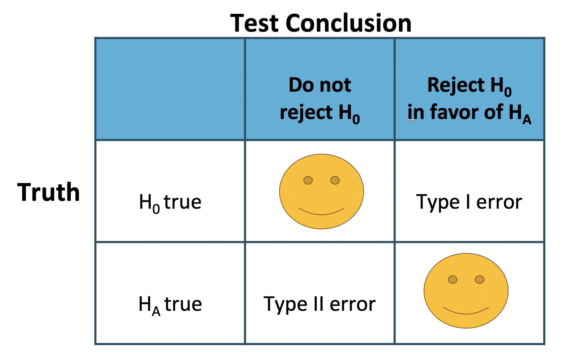
Because hypothesis tests are based on sample data, errors are possible. The two most common are Type I and Type II errors.

Type I Error (\(\alpha\)): Rejecting \(H_0\) when it is actually true (false positive).
Type II Error (\(\beta\)): Failing to reject \(H_0\) when \(H_a\) is actually true (false negative).

Courtroom Analogy for Hypothesis Testing

The logic of hypothesis testing is similar to a criminal trial:
- The defendant is presumed innocent (analogous to assuming \(H_0\) is true).
- Evidence (sample data) is presented.
- The jury decides whether there is enough evidence to “reject innocence” (reject \(H_0\)).

Truth	Fail to convict (fail to reject \(H_0\))	Convict (reject \(H_0\))
Defendant is innocent (\(H_0\) true)	Correct	Type I Error
Defendant is guilty (\(H_a\) true)	Type II Error	Correct

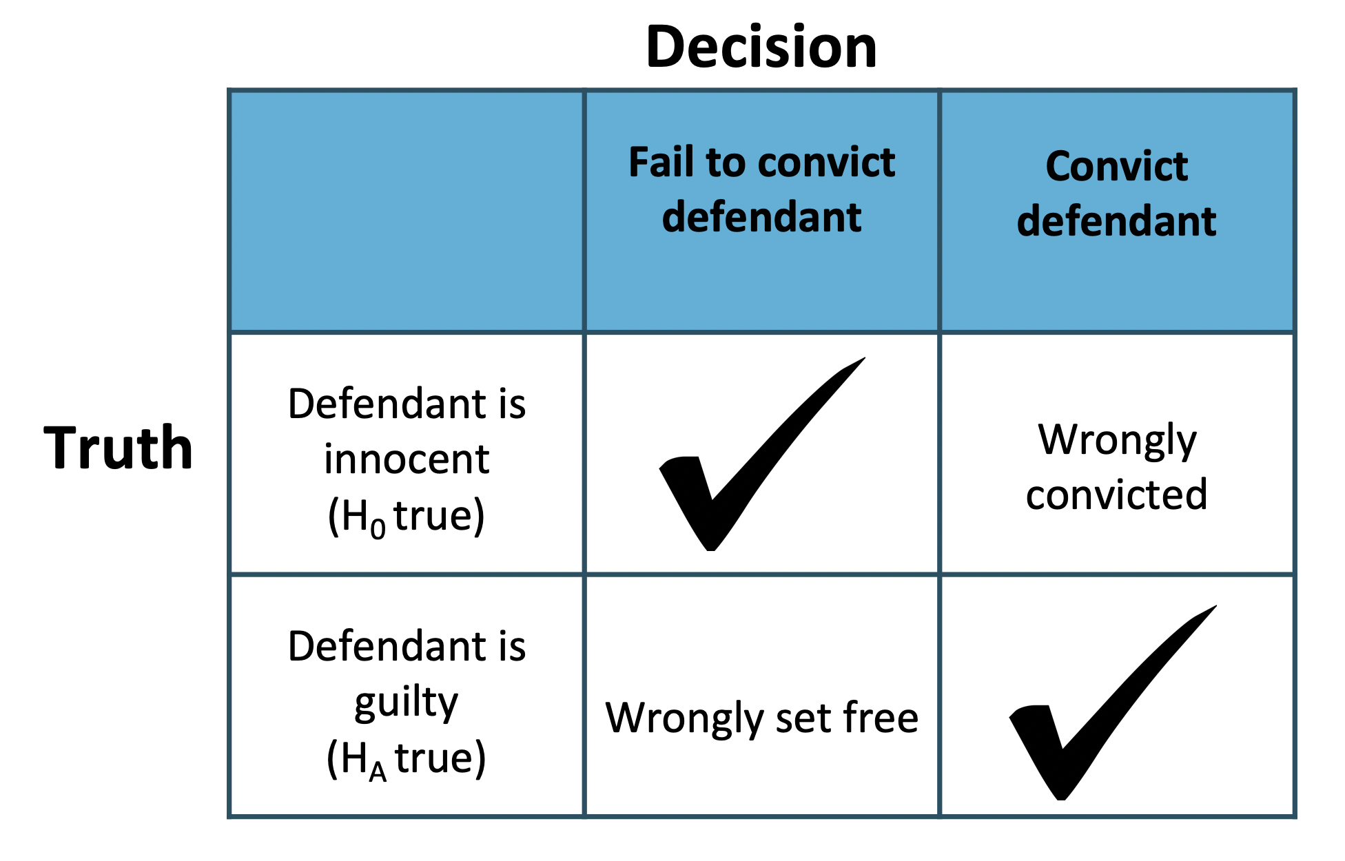
The significance level (\(\alpha\)) represents the risk of a Type I error, i.e., the probability of rejecting \(H_0\) when it is true.

One-Sided vs Two-Sided Tests

Two-sided test: Detects differences in either direction (\(H_a: p \ne p_0\)).
One-sided test: Focuses on a specific direction (\(H_a: p > p_0\) or \(H_a: p < p_0\)).

Important:
The direction of the test must be decided before examining the data. Choosing a one-tailed test after seeing results doubles the true error rate (e.g., from 5% to 10%), invalidating the conclusions.

Relationship Between Confidence Intervals and Hypothesis Testing

A two-tailed test with significance level \(\alpha\) corresponds to a \((1 - \alpha) \times 100\%\) confidence interval.
If the hypothesized value \(p_0\) lies outside the interval → reject \(H_0\).
If it lies inside → fail to reject \(H_0\).

3.3.3 Knowledge Check

3.3.4 Solved Exercises

The following examples explore hypothesis testing for proportions.

Exercise 1 Formulate null and alternative hypotheses

(a) A company claims that the proportion of customers filing complaints is now less than 0.10.

(b) An inspector wants to determine if the defect rate for a batch of screws exceeds 4%.

(c) A university official believes that the proportion of students working part-time has changed from 0.30 compared to last year.

Solution

\[ H_0: p = 0.10, \quad H_A: p < 0.10 \]
\[ H_0: p = 0.04, \quad H_A: p > 0.04 \]
\[ H_0: p = 0.30, \quad H_A: p \ne 0.30 \]

Exercise 2 Sample test for proportion

A census recorded that 15% of families lived below the poverty line five years ago. A random sample of 500 families today shows 90 families below the poverty line. Test whether the current proportion has changed. Use significance level \(\alpha = 0.05\).

(a) Formulate the hypotheses.
(b) Compute the sample proportion \(\hat{p}\).
(c) Compute the test statistic \(z = \frac{\hat{p} - p_0}{\sqrt{p_0(1-p_0)/n}}\).
(d) Compute the p-value.
(e) Draw a conclusion.

Solution

\[ H_0: p = 0.15, \quad H_A: p \ne 0.15 \]
Sample proportion:
\[ \hat{p} = \frac{90}{500} = 0.18 \]
Test statistic:
\[ z = \frac{0.18 - 0.15}{\sqrt{0.15 \times 0.85 / 500}} = \frac{0.03}{0.01595} \approx 1.88 \]
Two-tailed p-value:
\[ p\text{-value} = 2 \times P(Z > 1.88) \approx 2 \times 0.030 \approx 0.06 \]
Conclusion: Since \(p\text{-value} = 0.06 > 0.05\), we fail to reject \(H_0\). There is insufficient evidence to conclude that the proportion has changed.

# Exercise 2
p0 <- 0.15
n <- 500
x <- 90
alpha <- 0.05

# (a)
cat("H0: p =", p0, ", HA: p != ", p0, "\n")

## H0: p = 0.15 , HA: p !=  0.15

# (b) sample proportion
p_hat <- x / n
cat("Sample proportion (p_hat):", p_hat, "\n")

## Sample proportion (p_hat): 0.18

# (c) test statistic z
z <- (p_hat - p0) / sqrt(p0 * (1 - p0) / n)
cat("Test statistic (z):", z, "\n")

## Test statistic (z): 1.878673

# (d) p-value two-tailed
p_value <- 2 * (1 - pnorm(abs(z)))
cat("p-value:", p_value, "\n")

## p-value: 0.06028917

# (e) conclusion
if (p_value < alpha) {
  cat("Reject H0: evidence suggests proportion has changed.\n")
} else {
  cat("Fail to reject H0: insufficient evidence to say proportion changed.\n")
}

## Fail to reject H0: insufficient evidence to say proportion changed.

Exercise 3 Another sample proportion test

A school claims that 40% of students participate in extracurricular activities. A survey of 150 students finds 65 participate.

(a) Formulate hypotheses.
(b) Compute \(\hat{p}\).
(c) Compute the test statistic.
(d) Compute the p-value.
(e) State conclusion at \(\alpha = 0.05\).

Solution

\[ H_0: p = 0.40, \quad H_A: p \ne 0.40 \]
Sample proportion:
\[ \hat{p} = \frac{65}{150} \approx 0.4333 \]
Test statistic:
\[ z = \frac{0.4333 - 0.40}{\sqrt{0.4 \cdot 0.6 / 150}} = \frac{0.0333}{0.040} \approx 0.83 \]
Two-tailed p-value:
\[ p\text{-value} = 2 \times P(Z > 0.83) \approx 2 \times 0.203 \approx 0.406 \]
Conclusion: Since \(p\text{-value} = 0.406 > 0.05\), we fail to reject \(H_0\). There is no evidence that the proportion differs from 40%.

# Exercise 3
p0 <- 0.40
n <- 150
x <- 65
alpha <- 0.05

# (a)
cat("H0: p =", p0, ", HA: p != ", p0, "\n")

## H0: p = 0.4 , HA: p !=  0.4

# (b)
p_hat <- x / n
cat("Sample proportion (p_hat):", round(p_hat, 4), "\n")

## Sample proportion (p_hat): 0.4333

# (c)
z <- (p_hat - p0) / sqrt(p0 * (1 - p0) / n)
cat("Test statistic (z):", round(z, 4), "\n")

## Test statistic (z): 0.8333

# (d)
p_value <- 2 * (1 - pnorm(abs(z)))
cat("p-value:", round(p_value, 4), "\n")

## p-value: 0.4047

# (e)
if (p_value < alpha) {
  cat("Reject H0: evidence suggests proportion differs from 0.40.\n")
} else {
  cat("Fail to reject H0: insufficient evidence of difference.\n")
}

## Fail to reject H0: insufficient evidence of difference.

Exercise 4 One-sided hypothesis test

A factory claims that fewer than 5% of its products are defective. A random sample of 200 products reveals 8 defective items.

(a) Formulate hypotheses.
(b) Compute \(\hat{p}\).
(c) Compute the test statistic.
(d) Compute the p-value.
(e) Draw a conclusion.

Solution

\[ H_0: p = 0.05, \quad H_A: p > 0.05 \]
Sample proportion:
\[ \hat{p} = \frac{8}{200} = 0.04 \]
Test statistic:
\[ z = \frac{0.04 - 0.05}{\sqrt{0.05 \cdot 0.95 / 200}} = \frac{-0.01}{0.0154} \approx -0.65 \]
One-tailed p-value (right-tailed test):
\[ P(Z > -0.65) = 0.742 \]
Conclusion: Since \(p\text{-value} = 0.742 > 0.05\), fail to reject \(H_0\). There is insufficient evidence to claim that defect rate exceeds 5%.

# Exercise 4
p0 <- 0.05
n <- 200
x <- 8
alpha <- 0.05

# (a)
cat("H0: p =", p0, ", HA: p > ", p0, "\n")

## H0: p = 0.05 , HA: p >  0.05

# (b)
p_hat <- x / n
cat("Sample proportion (p_hat):", p_hat, "\n")

## Sample proportion (p_hat): 0.04

# (c)
z <- (p_hat - p0) / sqrt(p0 * (1 - p0) / n)
cat("Test statistic (z):", round(z, 4), "\n")

## Test statistic (z): -0.6489

# (d) one-tailed p-value (right tail)
p_value <- 1 - pnorm(z)
cat("p-value:", round(p_value, 4), "\n")

## p-value: 0.7418

# (e)
if (p_value < alpha) {
  cat("Reject H0: evidence suggests defect rate exceeds 5%.\n")
} else {
  cat("Fail to reject H0: insufficient evidence defect rate exceeds 5%.\n")
}

## Fail to reject H0: insufficient evidence defect rate exceeds 5%.

Exercise 5 Using significance for world health knowledge

In a multiple-choice question about vaccination coverage, 120 of 300 randomly sampled adults answered correctly. Assume random guessing would give 33.3% correct. Test at \(\alpha = 0.05\) whether adults perform better than random guessing.

(a) Hypotheses
(b) Sample proportion
(c) Test statistic
(d) p-value
(e) Conclusion

Solution

\[ H_0: p = 0.333, \quad H_A: p > 0.333 \]
Sample proportion:
\[ \hat{p} = \frac{120}{300} = 0.40 \]
Test statistic:
\[ z = \frac{0.40 - 0.333}{\sqrt{0.333 \cdot 0.667 / 300}} = \frac{0.067}{0.0273} \approx 2.45 \]
One-tailed p-value:
\[ P(Z > 2.45) \approx 0.0071 \]
Conclusion: Since \(p\text{-value} = 0.0071 < 0.05\), we reject \(H_0\). Adults perform significantly better than random guessing.

# Exercise 5
p0 <- 0.333
n <- 300
x <- 120
alpha <- 0.05

# (a)
cat("H0: p =", p0, ", HA: p > ", p0, "\n")

## H0: p = 0.333 , HA: p >  0.333

# (b)
p_hat <- x / n
cat("Sample proportion (p_hat):", p_hat, "\n")

## Sample proportion (p_hat): 0.4

# (c)
z <- (p_hat - p0) / sqrt(p0 * (1 - p0) / n)
cat("Test statistic (z):", round(z, 4), "\n")

## Test statistic (z): 2.4624

# (d)
p_value <- 1 - pnorm(z)
cat("p-value:", round(p_value, 4), "\n")

## p-value: 0.0069

# (e)
if (p_value < alpha) {
  cat("Reject H0: adults perform significantly better than random guessing.\n")
} else {
  cat("Fail to reject H0: insufficient evidence adults perform better than guessing.\n")
}

## Reject H0: adults perform significantly better than random guessing.