2.3 Binomial Distribution
2.3.1 Objectives
By the end of this unit, students will be able to:
- Identify when the conditions apply for the Binomial distribution to be used.
- Apply the Binomial distribution to model counts resulting from binary trials.
2.3.2 Overview
Binomial Distribution Condition
Conditions to be satisfied for a Binomial Variable Distribution with a fixed number of trials \(n\):
- The trials are independent
- Each trial has two possible outcomes classified as success or failure
- The probability of a success \(p\) is the same for each trial
Probability Mean and Standard Deviation
For a binomial random variable \(X\) with \(n\) trials and the probability of a single trial being a success \(p\), the probability of observing exactly \(k\) successes is
\[ P(X = k) = \binom{n}{k} p^k (1-p)^{n-k} = \frac{n!}{k!(n-k)!} p^k (1-p)^{n-k} \quad (k = 0, 1, \ldots, n) \]
Where: - \(n! = 1 \times 2 \times \cdots \times n\) - \(0! = 1\) - \(\binom{n}{k} = \frac{n!}{k!(n-k)!}\) (read as “n choose k”, also called the combination coefficient)
The probability of at most \(k\) successes is given by \[\displaystyle{\mathbb{P}\left[X \leq k\right] = \sum_{i=0}^{k}{\binom{n}{i}\cdot p^i\left(1 - p\right)^{n-i}} \approx \tt{pbinom(k, n, p)}}\]
In the equations above, \(\binom{n}{k} = \frac{n!}{k!\left(n-k\right)!}\) counts the number of ways to arrange the \(k\) successes amongst the \(n\) trials. That being said, the R functionality, dbinom() and pbinom() allow us to bypass the messy formulas – but you’ll still need to know what these functions do in order to use them correctly!
Tip: We need to use the binomial distribution to find probabilities associated with numbers of successful (or failing) outcomes in which we do not know for certain the trials on which the successes (or failures) occur
Mean: \(\mu = np\)
Standard deviation: \(\sigma = \sqrt{np(1-p)}\)
Observations that are more than 2 standard deviations away from the mean are considered unusual:
Unusual if outside of \(\mu - 2\sigma\) and \(\mu + 2\sigma\)
Shape of Binomial Distribution
- For \(p < 0.5\): skew to the left
- For \(p > 0.5\): skew to the right
- For \(p = 0.5\): symmetric (centered at \(\mu\))
- For large \(n\), if \(np \geq 10\) and \(n(1-p) \geq 10\), the graph is approximately bell-shaped.
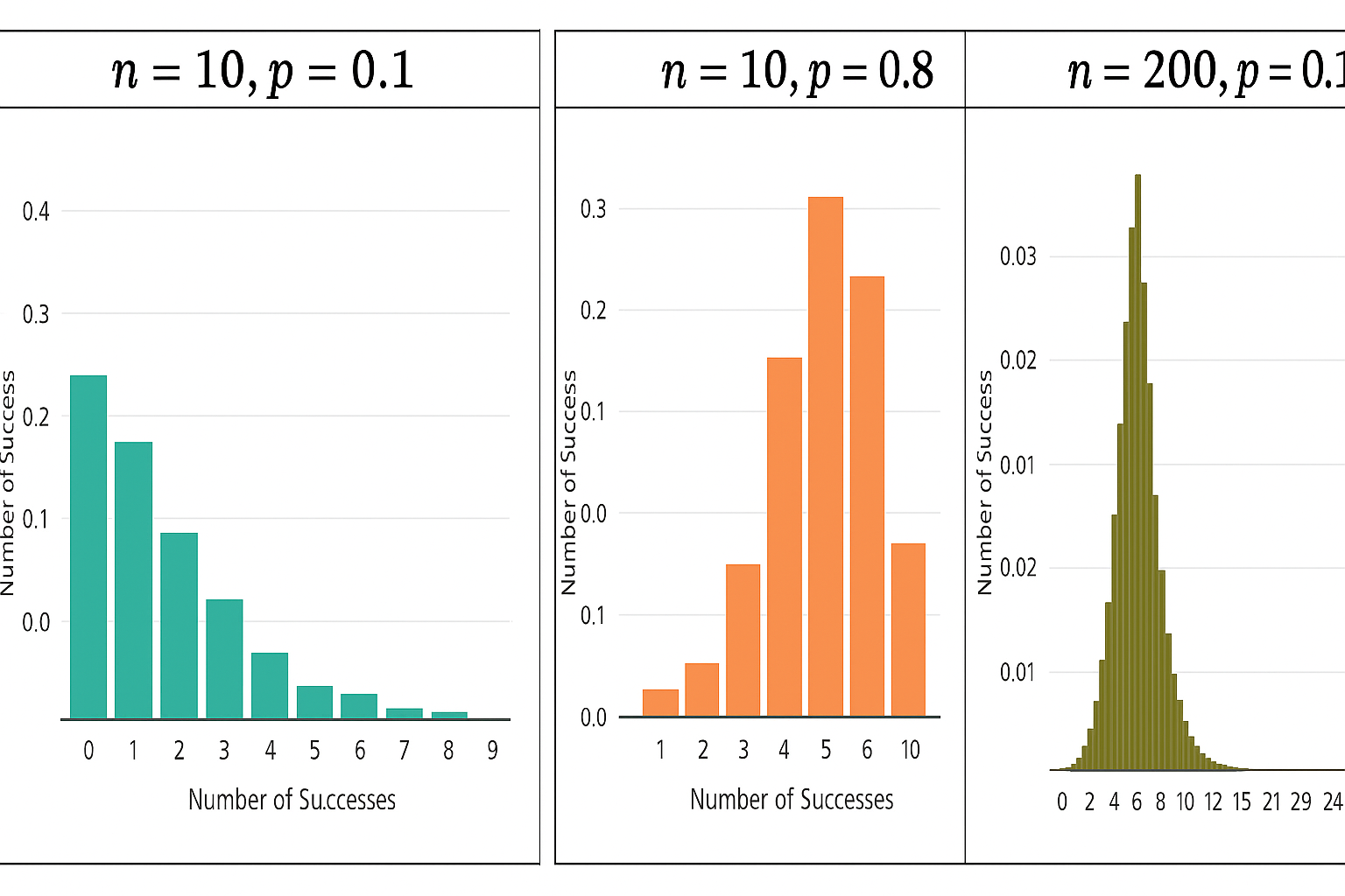
(Generated using online app https://istats.shinyapps.io/BinomialDist/)
Using R
For \(P(X = k)\):
dbinom(k, n, p)For \(P(X \leq k) = P(X < k+1) = P(X = 0) + P(X = 1) + \cdots + P(X = k)\):
pbinom(k, n, p, lower.tail = TRUE)(thelower.tail = TRUEcan be omitted)For \(P(X > k) = P(X \geq k+1) = 1 - P(X \leq k) = P(X = k+1) + \cdots + P(X = n)\):
pbinom(k, n, p, lower.tail = FALSE)For \(n!\):
factorial(n)For \(\binom{n}{k}\):
choose(n, k)
2.3.4 Solved Exercises
Exercise 1 How many ways can we select 3 volunteers from a group of 8?
\[ \binom{8}{3} = \frac{8!}{3!(8-3)!} = \frac{8 \times 7 \times 6}{3 \times 2 \times 1} = 56 \]
Exercise 2 (Combination Formula)
Survey five randomly selected employees and record the outcomes as “Y” (yes, they work remotely) or “N” (no, they don’t). Fill in the table below.
| # of “Y” | Outcomes (list all) | # of outcomes | \(\displaystyle \binom{5}{k} = \frac{5!}{k!(5-k)!}\) |
|---|---|---|---|
| \(k = 0\) | NNNNN | 1 | 1 |
| \(k = 1\) | YNNNN, NYNNN, NNYNN, NNNYN, NNNNY | 5 | 5 |
| \(k = 2\) | YYNNN, YNYNN, YNNYN, YNNNY, NYYNN, NYNYN, NYNNY, NNYYN, NNYNY, NNNYY | 10 | 10 |
| \(k = 3\) | YYYNN, YYNYN, YYNYY, YNYYN, YNYNY, YNNYY, NYYYY, NYYY, etc. | 10 | 10 |
| \(k = 4\) | YYYYN, YYYNY, YYNYY, YNYYY, NYYYY | 5 | 5 |
| \(k = 5\) | YYYYY | 1 | 1 |
Exercise 3
Find the probability of success of the Bernoulli trial with \(n\) trials, success probability \(p\), and the number of successes \(k\):
\[ P(X = k) = \binom{n}{k} p^k (1-p)^{n-k} \]
For example:
\[ \begin{aligned} P(X = 1) &= \binom{4}{1}(0.4)^1(0.6)^3 = 4(0.4)(0.216) = 0.3456 \\ P(X = 3) &= \binom{5}{3}(0.25)^3(0.75)^2 = 10(0.0156)(0.5625) = 0.0879 \end{aligned} \]
Exercise 4
For a binomial distribution with \(n = 5\), \(p = 0.6\).
(Assume that 60% of customers prefer online shopping.)
(a) Formula for computing the probability of getting exactly \(k\) successes:
\[ P(X = k) = \binom{n}{k}p^k(1-p)^{n-k} = \frac{n!}{k!(n-k)!}p^k(1-p)^{n-k}, \quad k = 0,1,\dots,n \]
(b) Distribution table (rounded to 4 decimals):
| \(X\) | \(P(X = k)\) | \(P(X \le k)\) |
|---|---|---|
| 0 | 0.0102 | 0.0102 |
| 1 | 0.0768 | 0.0870 |
| 2 | 0.2304 | 0.3174 |
| 3 | 0.3456 | 0.6630 |
| 4 | 0.2592 | 0.9222 |
| 5 | 0.0778 | 1.0000 |
| Total | 1.0000 |
(c) Expected value:
\[ E[X] = n p = 5(0.6) = 3 \]
(d) Standard deviation:
\[ \sigma = \sqrt{n p (1-p)} = \sqrt{5(0.6)(0.4)} = \sqrt{1.2} = 1.095 \]
Exercise 5
About 40% of residents in a city own a cat. Suppose 15 residents are randomly selected.
(a) Exactly five own a cat:
\[ P(X = 5) = \binom{15}{5}(0.40)^5(0.60)^{10} = 0.1859 \]
(b) Exactly twelve do not own a cat:
\[ P(X = 12) = \binom{15}{12}(0.60)^{12}(0.40)^3 = 0.0284 \]
(c) At least three own a cat:
\[ P(X \ge 3) = 1 - P(X \le 2) \]
(d) At most four own a cat:
\[ P(X \le 4) = \sum_{x=0}^{4} P(X = x) \]
(e) Between six and ten (inclusive) own a cat:
\[ P(6 \le X \le 10) = P(X \le 10) - P(X \le 5) \]
(f) Expected number of residents who own a cat:
\[ E[X] = n p = 15(0.4) = 6 \]
(g) Is it unusual if 13 out of 15 own a cat?
\[ P(X = 13) = \binom{15}{13}(0.40)^{13}(0.60)^2 \]
If this probability is very low (e.g., below 0.05), the event may be considered unusual.
(h) Is it unusual if 5 out of 15 own a cat?
\[ P(X = 5) = \binom{15}{5}(0.40)^5(0.60)^{10} \]
If the probability is moderate or higher (e.g., above 0.05), it would not be considered unusual.