2.4 Normal Distribution
2.4.1 Objectives
By the end of this unit, students will be able to:
- Understand the notion and characteristics of continuous probability distributions.
- Use the normal distribution to model continuous random variables.
2.4.2 Overview
2.4.2.1 Introduction
The Normal distribution, also known as the Gaussian distribution, is the most widely used continuous probability distribution in statistics.
It describes many natural and social phenomena such as human height, IQ scores, and measurement errors, which tend to cluster symmetrically around a central mean.
A random variable \(X\) that follows a normal distribution with mean \(\mu\) and standard deviation \(\sigma\) is written as:
\[ X \sim N(\mu, \sigma) \]
Its probability density function (PDF) is given by:
\[ f(x) = \frac{1}{\sqrt{2\pi\sigma^2}} e^{-\frac{1}{2}\left(\frac{x - \mu}{\sigma}\right)^2} \]
This bell-shaped curve is symmetric about the mean \(\mu\), and values close to the mean occur more frequently than those farther away.
2.4.2.2 Characteristics of the Normal Distribution
For \(X \sim N(\mu, \sigma)\):
- The total area under the curve equals 1, representing total probability.
- The curve is symmetrical about the mean \(\mu\).
- The mean, median, and mode are equal.
- The standard deviation (\(\sigma\)) determines the spread or width of the curve:
- Large \(\sigma\): flatter, wider curve.
- Small \(\sigma\): narrower, taller curve.
- Large \(\sigma\): flatter, wider curve.
- Probabilities are found by measuring the area under the curve, not by individual points (since \(P(X = k) = 0\)).
Insert Image: Diagram showing the symmetry and area of a normal curve with 50% on each side of the mean.
2.4.2.3 The Empirical Rule (68–95–99.7 Rule)
The Empirical Rule summarizes how data are distributed in a normal curve:
| Range from Mean | Approx. % of Data | Interpretation |
|---|---|---|
| \(\mu \pm 1\sigma\) | 68% | About two-thirds of values fall within 1 standard deviation |
| \(\mu \pm 2\sigma\) | 95% | About 95% of values fall within 2 standard deviations |
| \(\mu \pm 3\sigma\) | 99.7% | Almost all values fall within 3 standard deviations |
Insert Image: A normal curve shaded to show 68%, 95%, and 99.7% regions.
2.4.2.4 The Standard Normal Distribution and Z-Scores
To compare data from different normal distributions, we standardize observations using a z-score, which converts any normal variable into a standard normal distribution:
\[ Z = \frac{X - \mu}{\sigma} \] where \(Z \sim N(0, 1)\).
A z-score indicates how many standard deviations an observation \(X\) lies from the mean:
- \(z > 0\): above the mean
- \(z < 0\): below the mean
- Large |z| values: far into the tails (unusual or rare observations)
Insert Image: Standard normal curve labeled with z-scores (-3 to +3).
2.4.2.5 Example: Comparing Test Scores
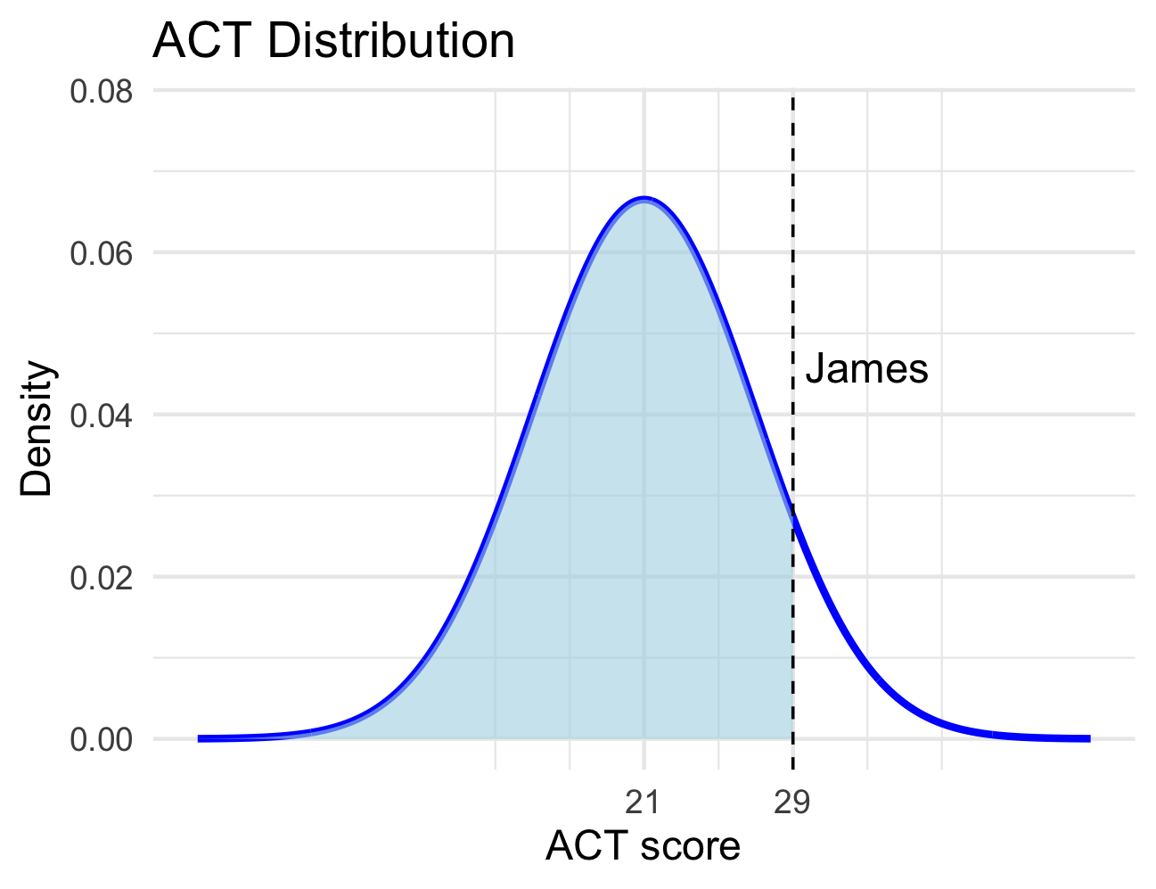
Suppose two students took different standardized exams: - SAT: \(\mu = 1050, \sigma = 200\) - ACT: \(\mu = 21, \sigma = 6\)
Maria scored 1350 on the SAT, and James scored 29 on the ACT.
Their standardized z-scores are:
\[ z_{Maria} = \frac{1350 - 1050}{200} = 1.58, \quad z_{James} = \frac{29 - 21}{6} = 1.76 \]
Because James’s z-score is higher, he performed better relative to his group.
Maria’s percentile corresponds to the shaded area in the distribution below:

’s percentile corresponds to the shaded area in the distribution below:
There are many ways to compute percentiles. Before the widespread availability of statistical software, people converted observed values to \(z\)-scores and then looked up the percentile in a table. Luckily R provides nice functionality for computing percentiles.
For these first few questions I’ll draw pictures for you, but you should be prepared to draw your own shortly.
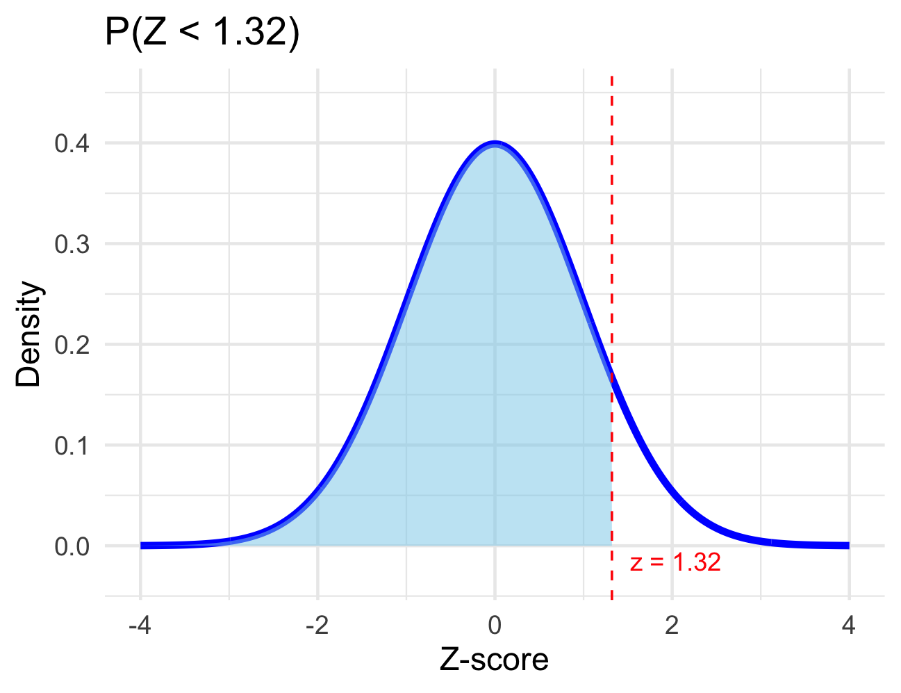
Question 1: Remember that \(Z\sim N\left(\mu = 0, \sigma = 1\right)\).
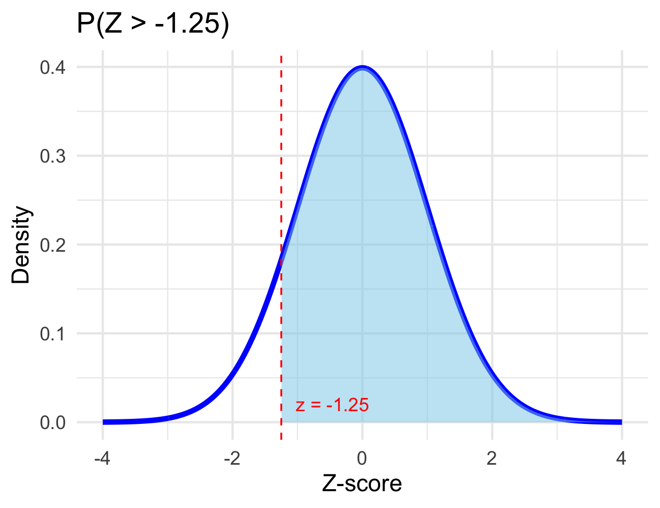
Question 2: Find \(\mathbb{P}\left[Z > \right.\) \(\left.\right]\).
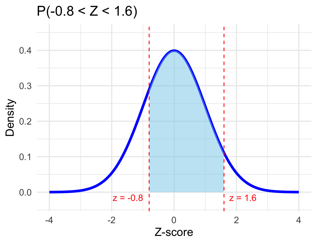
Question 3: Find \(\mathbb{P}\left[\right.\) \(< Z <\) \(\left.\right]\).
Through the last three problems you only worked with the standard normal distribution – that’s the \(Z\)-distribution, which is \(N\left(\mu = 0, \sigma = 1\right)\). We can find probabilities from arbitrary normal distributions (normal distributions with any mean and any standard deviation) using R’s ‘pnorm()’ functionality – just supply the appropriate ‘mean’ and ‘sd’ arguments to ‘pnorm()’ instead of the 0 and 1 that we passed earlier.
2.4.4 Solved Exercises
Exercise 1 For \(Z \sim N(0, 1)\) (the standard normal distribution, mean = 0, standard deviation = 1), use R to find the probability and sketch the region that represents the probability.
- \(P(Z < -1.2)\)
- \(P(Z > 2.1)\)
- \(P(-0.8 < Z < 1.5)\)
- \(P(|Z| < 1.8)\)
- \(P(Z > 0.75)\)
Solution
## [1] 0.1150697## [1] 0.01786442## [1] 0.7213374## [1] 0.9281394## [1] 0.2266274Exercise 2 For \(X \sim N(4, 1.5)\) (a normal distribution with mean = 4 and standard deviation = 1.5), use R to find the probability and sketch the region that represents the probability.
- \(P(X < 3)\)
- \(P(X > 6)\)
- \(P(3 < X < 5.5)\)
Solution
## [1] 0.2524925## [1] 0.09121122## [1] 0.5888522Exercise 3 For \(X \sim N(4, 1.5)\), compute the z-score of the given x-values:
- \(x = 3\)
- \(x = 4\)
- \(x = 5.5\)
Solution
mu <- 4
sigma <- 1.5
z1 <- (3 - mu) / sigma
z2 <- (4 - mu) / sigma
z3 <- (5.5 - mu) / sigma
z1; z2; z3
## [1] -0.6666667## [1] 0## [1] 1Exercise 4
State the Empirical Rule.
Use R to verify the Empirical Rule: find \(P(|Z| < 1)\), \(P(|Z| < 2)\), and \(P(|Z| < 3)\).
Solution
(a) Empirical Rule:
About 68% of data lies within 1 standard deviation of the mean.
About 95% lies within 2 standard deviations.
About 99.7% lies within 3 standard deviations.
## [1] 0.6826895## [1] 0.9544997## [1] 0.9973002Exercise 5
The weights of newborn babies follow a normal distribution with a mean of 3.2 kg and standard deviation of 0.5 kg. Find the probability that a randomly chosen baby weighs:
Over 3.8 kg
Less than 2.6 kg
Between 2.8 kg and 3.6 kg
Solution
## [1] 0.1150697## [1] 0.1150697## [1] 0.5762892Exercise 6 The weights of newborn babies follow a normal distribution with a mean of 3.2 kg and standard deviation of 0.5 kg.
What is the cutoff weight for the lowest 25% of babies? (Round to 1 decimal place.)
What is the cutoff weight for the highest 5% of babies? (Round to 1 decimal place.)
Solution
## [1] 2.862755## [1] 4.022427Exercise 7
The daily time (in hours) students spend studying follows a normal distribution with a mean of 5.4 hours and standard deviation of 1.1 hours.
Find the (standardized) z-score corresponding to a student who studies 4.2 hours.
Solution
## [1] -1.090909Exercise 8
Maria scored 76 on a statistics test with a mean of 70 and a standard deviation of 5. Liam scored 88 on a chemistry test with a mean of 82 and a standard deviation of 4. Find the z-scores for Maria’s and Liam’s test results and determine who performed better relative to their class.
Solution
## [1] 1.2## [1] 1.5Exercise 9
The score data of the verbal portion of the Graduate Record Examination (GRE) is approximately normally distributed with a mean of 475 points and a standard deviation of 108 points. Fill in the following blanks: approximately
(a) 68% of students who took the verbal portion of the GRE scored between _______ and ________
(b) 95% of students who took the verbal portion of the GRE scored between ______ and ________
(c) 99.7% of students who took the verbal portion of the GRE scored between ______ and ________
Solution
According to the Empirical Rule:
\[ \begin{aligned} 68\% &:\ \mu \pm 1\sigma \\ 95\% &:\ \mu \pm 2\sigma \\ 99.7\% &:\ \mu \pm 3\sigma \end{aligned} \]
Given:
\(\mu = 475,\ \sigma = 108\)
Compute each range:
mu <- 475
sigma <- 108

# (a) 68% within 1 standard deviation
low_68 <- mu - sigma
high_68 <- mu + sigma

# (b) 95% within 2 standard deviations
low_95 <- mu - 2 * sigma
high_95 <- mu + 2 * sigma

# (c) 99.7% within 3 standard deviations
low_997 <- mu - 3 * sigma
high_997 <- mu + 3 * sigma

low_68; high_68
## [1] 367## [1] 583## [1] 259## [1] 691## [1] 151## [1] 799