1.1 Data Types
1.1.1 Objectives
By the end of this section, students will be able to:
- Understand the importance of statistical methods for answering research questions using data.
- Identify different types of data that can be analyzed using statistical methods.
- Describe basic sampling principles and strategies for the purpose of collecting data for research studies.
- Describe basic principles of designing research experiments.
1.1.2 Overview
In this section, we focus on how to classify variables into numerical or categorical types. This classification is critical, as it guides which summary statistics we compute, what types of graphs we construct, and which statistical methods are appropriate for answering research questions.
There are two broad types of variables:
- Numerical (quantitative): values are numbers where arithmetic operations such as addition, subtraction, or averaging are meaningful.
- Categorical (qualitative): values place observations into distinct groups or categories. Categories may sometimes be coded with numbers (e.g., Likert scales from 1 = strongly disagree to 5 = strongly agree), but these codes serve only as labels — it would not be sensible to add or average them.
1.1.2.1 Numerical Data
Numerical variables can be divided into continuous and discrete types:
- Continuous variables are typically measured on a scale and can take on infinitely many values within a range (e.g., height or weight).
- Discrete variables arise when the values are countable or finite (e.g., number of pets in a household).
When deciding if a variable is continuous or discrete, consider its true nature rather than its recorded form. For example, height is inherently continuous, even though it is often rounded to the nearest inch or centimeter, which may make it appear discrete.
1.1.2.2 Categorical Data
Categorical variables can be further classified as:
- Ordinal: categories follow a natural ordering (e.g., survey ratings from “very unsatisfied” to “very satisfied”).
- Nominal: categories with no inherent order (e.g., blood type, whether someone consumes caffeine).
1.1.2.3 Data Collection Principles
Statistical work often involves using a sample to make generalizations about a population.
- Population: the entire group we want to draw conclusions about.
- Sample: the subset of the population actually observed.
Key Idea: Results based on a sample can only be generalized to the population if the sample is representative.
Why not rely on a census?
- A census is resource-intensive, requiring far more time and money than sampling.
- Some individuals are difficult to contact, and missing them introduces bias (e.g., undocumented immigrants in U.S. census data).
- Populations change over time, so even a perfectly conducted census quickly becomes outdated.
Because of these challenges, sampling is the more practical and effective approach.
1.1.2.4 Sampling Is Natural
Sampling is similar to tasting food while cooking. A spoonful (the sample) helps us infer the taste of the whole pot (the population). However, for the inference to be valid, the spoonful must be representative. If you only taste the top layer where salt has not mixed evenly, you get a misleading impression. Stirring the pot before tasting mimics proper sampling, ensuring the spoonful reflects the whole.
1.1.2.5 Steps in Sampling
- Identify the research question and the population of interest.
- Collect reliable data that serve the research goal.
Key terms:
- Population vs. Sample: The population is the full group of interest; the sample is the group observed.
- Parameter vs. Statistic: A parameter describes the population (usually unknown). A statistic describes the sample (calculated from data).
- Observational Study vs. Experiment:
- Observational study: data are collected without interference.
- Experiment: subjects are randomly assigned to treatments so causal relationships can be investigated.
1.1.2.6 Sampling Methods
Four widely used probability sampling designs are:
- Simple Random Sample (SRS): each case has an equal chance of being selected, similar to drawing names from a hat.

- Stratified Sample: population is divided into homogeneous strata, and random samples are taken from each.

- Cluster Sample: population is split into heterogeneous clusters, and some entire clusters are sampled.
- Multistage Sample: begins like cluster sampling, but then takes random samples within selected clusters.
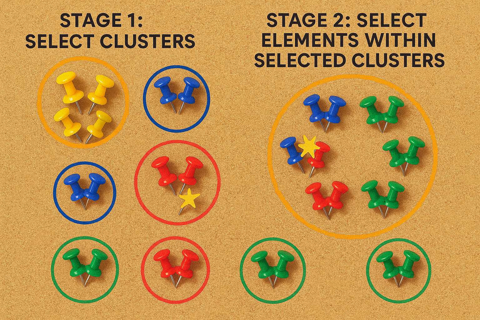
Note: Cluster and multistage methods are often chosen for cost and convenience, such as sampling a few regions in a city rather than the entire city.
Convenience Samples: The most common — but least reliable — approach is to sample individuals who are easy to reach. This often leads to bias. Famous examples include the 1936 Literary Digest poll, which incorrectly predicted the U.S. presidential election, and many election polls affected by convenience sampling errors.
1.1.2.7 Practice Scenarios
- Determine which method: A company samples 50 addresses from each Boston zip code to send coupons. → Stratified sample.
- Choose the worst method: A school district surveys a few entire neighborhoods to estimate student SES, even though neighborhoods differ widely. → Cluster sample is misleading here.
1.1.2.8 Experimental Design
Beyond sampling, data can be collected through observational studies or experiments:
- Observational study: researchers do not interfere; only associations can be studied.
- Experiment: researchers randomly assign treatments, enabling causal conclusions.
Four principles of experimental design:
1. Control – use treatment and control groups for comparison.
2. Randomization – randomly assign subjects to groups.
3. Replication – use a sufficiently large sample or repeat the study.
4. Blocking – group similar individuals before randomization to reduce variability.
1.1.2.9 Explanatory and Response Variables
- Explanatory variable (x): the factor believed to influence the outcome.
- Response variable (y): the outcome being measured.
Relationships can involve multiple explanatory variables.
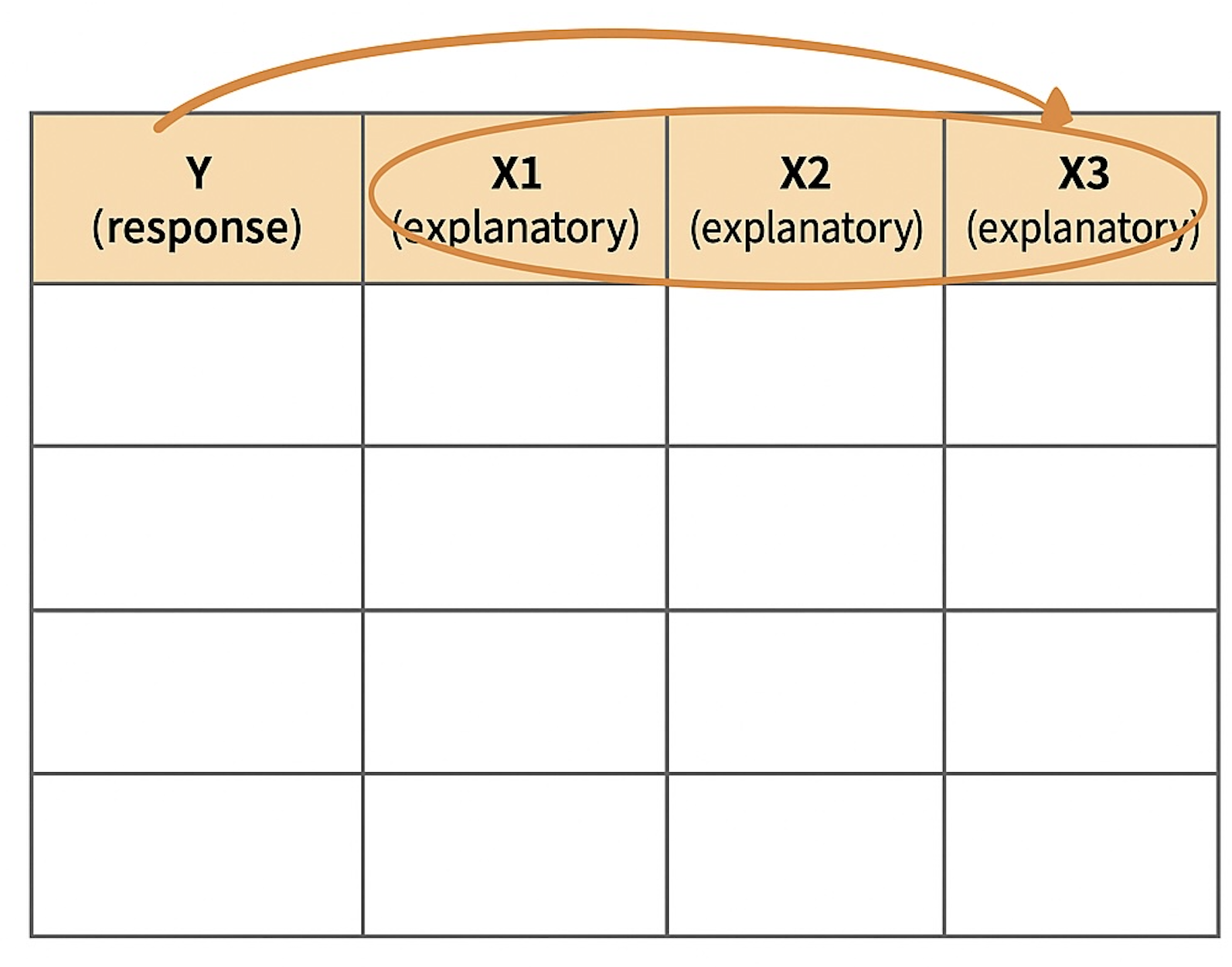
For example, studying the effect of calorie intake on heart health might also require accounting for age and exercise level.
1.1.4 Solved Exercises
Exercise 1. A middle school wanted to study whether extra tutoring in math helps improve quiz performance compared to regular study hall. A total of 166 students were randomly assigned to one of two groups: tutoring or study hall. Students in the tutoring group met with a teacher for 10 days, while the study hall group worked independently during that time. At the end of the 10-day period, students took a math quiz, and results were recorded as “Improved” or “Not Improved.” The distribution of responses is summarized below (with some cells missing numbers):
(for b), c), Round answers to within one hundredth of a percent)
| Improved quiz scores | ||||
|---|---|---|---|---|
| Yes | No | Total | ||
| Tutoring | 66 | 85 | ||
| Study hall | 65 | |||
| Total | 166 |
(a). Fill the blank cells in the above table.
(b). What percent of students in the tutoring group improved?
(c). What percent of students in the study hall group improved?
(d). In which group did a higher percentage improve?
(e). What is one other possible explanation for the observed difference besides the tutoring being effective?
Answer: (a).
| Improved quiz scores | ||||
|---|---|---|---|---|
| Yes | No | Total | ||
| Tutoring | 66 | 19 | 85 | |
| Study hall | 65 | 16 | 81 | |
| Total | 131 | 35 | 166 |
(b). 66 ÷ 85 = 77.65%
(c). 65 ÷ 81 = 80.25%
(d). The study hall group had a slightly higher percentage.
(e). Differences could be due to random variation or outside factors (e.g., students studying at home differently).
Exercise 2.
The following table displays data from a micro-lending company.
| loan.amount | interest.rate | term | grade | state | total.income | homeownership |
|---|---|---|---|---|---|---|
| 9000 | 7.12 | 36 | A | TX | 72000 | rent |
| 22000 | 10.01 | 60 | B | IL | 265000 | mortgage |
| 13000 | 6.45 | 36 | A | FL | 85000 | mortgage |
| … | … | … | … | … | … | … |
| 4500 | 8.22 | 36 | A | WA | 36000 | rent |
Variable descriptions
- loan.amount: Amount of the loan received, in US dollars.
- interest.rate: Interest rate on the loan, in an annual percentage.
- term: The length of the loan, always a whole number of months.
- grade: Loan grade (A through G), representing the loan quality and likelihood of repayment.
- state: US state where the borrower resides.
- total.income: Borrower’s total income, including any secondary income, in US dollars.
- homeownership: Indicates whether the person owns, owns with a mortgage, or rents.
Questions
- How many cases are in the data?
- Identify the types of variables.
Answer:
Each row is one case (one borrower/loan). There are as many cases as rows in the full dataset.
Variable types:
loan.amount: numerical (continuous)interest.rate: numerical (continuous, percentage)term: numerical (discrete, months)grade: categorical (ordinal: A–G)state: categorical (nominal: state abbreviations)total.income: numerical (continuous)homeownership: categorical (nominal: rent/mortgage/own)
Exercise 3. A school counselor wanted to test if practicing mindfulness during homeroom reduces stress and improves focus. Six hundred students aged 12–18 who reported stress were randomly split into two groups: one practiced mindfulness daily, the other did not. Students were scored on stress, focus, participation, and reliance on coping strategies on a 0–10 scale. On average, the mindfulness group reported lower stress and higher focus.
(a). What is the main research question?
(b). Who are the subjects, and how many are included?
(c). What are the variables? Classify them.
Answer:
(a). Does daily mindfulness practice reduce stress and improve focus in students?
(b). 600 middle and high school students, ages 12–18.
(c). Stress (numerical, discrete), focus (numerical, discrete), participation (categorical), reliance on coping strategies (categorical).
Exercise 4. A district study examined whether cafeteria air quality is linked to student absenteeism. Air quality levels were recorded daily in 15 cafeterias, and absence records were collected for 12,500 students between 2010 and 2014.
(a). Identify the population and the sample.
(b). Can the results be generalized? Can causal conclusions be made?
Answer:
(a). Population: All students in the district. Sample: The 12,500 students with recorded attendance matched to cafeteria air quality.
(b). Results may generalize if the cafeterias are representative. Because the study is observational, causality cannot be claimed.
Exercise 5. A PE teacher is interested in the average number of minutes students spend running during class. Match the vocabulary words (a-f) with the examples (1-6).
Examples:
- All 40 run times recorded from the students in the study.
- The 40 students who participated.
- All students at the school.
- The average run time of all students at the school.
- The run time of any one student.
- The average run time of the 40 students studied.
Vocabulary:
Data
Population
Variable
Sample
Parameter
Statistic
Answer:
1–a, 2–d, 3–b, 4–e, 5–c, 6–f
Exercise 6. (Observational Study or Experiment)
You would like to know whether eating breakfast before class affects test performance. One group is told to eat breakfast before a quiz, the other group skips. Is this an experiment or observational study?
GPA and part-time job status of seniors are recorded. Is this an experiment or observational study?
Answer:
(a). Experiment (researchers assign who eats breakfast).
(b). Observational study (no assignment, just data collection).
Exercise 7. A study looked at the effects of physical activity breaks on mood. Students were randomly assigned to: (1) no break, (2) app reminders to stretch plus a short daily movement video, or (3) two structured group exercise breaks per day. Participants were student volunteers at a high school in Boston. After 14 days, only group 3 showed consistent mood improvements.
(a). What type of study is this?
(b). Identify explanatory and response variables.
(c). Can results be generalized?
(d). Can causal claims be made?
(e). A school paper reports: “This proves exercise breaks boost mood.” How should this be revised?
Answer: (a). Experiment
(b). Explanatory: activity group (categorical, 3 levels). Response: mood (categorical/numerical scale).
(c). No — only volunteers were studied.
(d). Yes — experimental design supports causation.
(e). Replace “proves” with “provides evidence.”