```{r setup, include=FALSE} knitr::opts_chunk$set(echo = FALSE) ``` ```{r, echo=F, message=F, warning=F} library(readr) library(openintro) data(COL) ``` # Binomial distribution ## Experiment \alert{Suppose a health insurance company found that 70\% of the people they insure stay below their deductible in any given year. This means that 30\% of the people exceed their deductible. Suppose the insurance agency is considering a random sample of four individuals they insure. What is the chance exactly one of them will exceed the deductible and the other three will not?} ## Experiment Let's call these people Allen (A), Brittany (B), Caroline (C), and Damian (D). Each one of the four scenarios below will satisfy the condition of "exactly 1 of them refuses to administer the shock": \pause \centering{Scenario 1: $\frac{0.3}{(A) \textcolor{red}{ exceed}} \times \frac{0.7}{(B) \text{ }Not} \times \frac{0.7}{(C) \text{ }Not} \times \frac{0.7}{(D) \text{ }Not}=0.103$} \pause \centering{Scenario 2: $\frac{0.7}{(A) \text{ }Not } \times \frac{0.3}{(B)\textcolor{red}{ exceed}} \times \frac{0.7}{(C) \text{ }Not} \times \frac{0.7}{(D) \text{ }Not}=0.103$} \pause \centering{Scenario 3: $\frac{0.7}{(A) \text{ }Not } \times \frac{0.7}{(B) \text{ }Not} \times \frac{0.3}{(C)\textcolor{red}{ exceed}} \times \frac{0.7}{(D) \text{ }Not}=0.103$} \pause \centering{Scenario 4: $\frac{0.7}{(A) \text{ }Not } \times \frac{0.7}{(B) \text{ }Not} \times \frac{0.7}{(C)\text{ }Not} \times \frac{0.3}{(D) \textcolor{red}{ exceed}}=0.103$} \pause \raggedright The probability of exactly one 1 of 4 people refusing to administer the shock is the sum of all of these probabilities. \centering{$0.103+0.103+0.103+0.103 = 4 \times 0.103 = 0.412$} ## Binomial distribution The question from the prior slide asked for the probability of given number of successes, **k**, in a given number of trials, **n**, (k = 1 success in $n=4$ trials), and we calculated this probability as \centering{$\#$ of scenarios $\times$ P(single scenario)} \pause - $\#$ of scenarios: there is a less tedious way to figure it out, we'll get to that shortly... \pause - P(single scenario) $= p^k \cdot (1-p)^{(n-k)}$ \raggedright\small \alert{Note:} probability of success to the power of number of successes, probability of failure to the power of number of failures. \pause \normalsize The **Binomial distribution** describes the probability of having exactly $k$ successes in $n$ independent Bernoulli trials with probability of success $p$. ## Counting the \# of scenarios Earlier we wrote out all possible scenarios that fit the condition of exactly one person refusing to administer the shock. If $n$ was larger and/or $k$ was different than 1, for example, $n=9$ and $k=2$. \centering{\alert{RR}SSSSSSS} \pause \centering{S\alert{RR}SSSSSS} \pause \centering{SS\alert{RR}SSSSS} \centering{$\dots$} \centering{SS\alert{R}SS\alert{R}SSS} \centering{$\dots$} \centering{SSSSSSS\alert{RR}} \raggedright Writing out all possible scenarios would be incredibly tedious and prone to errors. ## Calculating the \# of scenarios The **choose function** is useful for calculating the number of ways to choose $k$ successes in $n$ trials. \centering{${n \choose k} = \frac{n!}{k! \cdot (n-k)!}$} \pause - $k=1, n=4: {4 \choose 1} = \frac{4!}{1!(4-1)!} = \frac{4 \times 3 \times 2 \times 1}{1 \times (3 \times 2 \times 1)} = 4$ \pause - $k=2, n=9: {9 \choose 2} = \frac{9!}{2!(9-2)!} = \frac{9 \times 8 \times 7!}{2 \times 1 \times 7!} = 36$ ## Properties of the choose function \alert{Which of the following is false?} A) There are $n$ ways of getting 1 success in $n$ trials, ${n \choose 1} = n$. B) There is only 1 way of getting $n$ successes in $n$ trials, ${n \choose n} = 1$. C) There is only 1 way of getting $n$ failures in $n$ trials, ${n \choose 0} = 1$. D) There are $n-1$ ways of getting $n-1$ successes in $n$ trials, ${n \choose n-1} = n-1$ ## Properties of the choose function \alert{Which of the following is false?} A) There are $n$ ways of getting 1 success in $n$ trials, ${n \choose 1} = n$. B) There is only 1 way of getting $n$ successes in $n$ trials, ${n \choose n} = 1$. C) There is only 1 way of getting $n$ failures in $n$ trials, ${n \choose 0} = 1$. D) \alert{There are $n-1$ ways of getting $n-1$ successes in $n$ trials, ${n \choose n-1} = n-1$} ## Binomial distribution If $p$ represents probability of success, $(1-p)$ represents probability of failure, $n$ represents number of independent trials, and $k$ represents number of successes \centering{P(k successes in n trials) = ${n \choose k}p^k(1-p)^{(n-k)}$} ## Practice \alert{Which of the following is not a condition that needs to be met for the binomial distribution to be applicable?} A) The trials must be independent. B) The number of trials, $n$, must be fixed. C) Each trial outcome must be classified as a success or a failure. D) The number of desired successes, $k$, must be greater than the number of trials. E) The probability of success, $p$, must be the same for each trial. ## Practice \alert{Which of the following is not a condition that needs to be met for the binomial distribution to be applicable?} A) The trials must be independent. B) The number of trials, $n$, must be fixed. C) Each trial outcome must be classified as a success or a failure. D) \alert{The number of desired successes, $k$, must be greater than the number of trials.} E) The probability of success, $p$, must be the same for each trial. ## Practice \alert{A 2012 Gallup survey suggests that 26.2\% of Americans are obese. Among a random sample of 10 Americans, what is the probability that exactly 8 are obese?} A) Pretty high B) Pretty low ## Practice \alert{A 2012 Gallup survey suggests that 26.2\% of Americans are obese. Among a random sample of 10 Americans, what is the probability that exactly 8 are obese?} A) Pretty high B) \alert{Pretty low} ## Practice \alert{A 2012 Gallup survey suggests that 26.2\% of Americans are obese. Among a random sample of 10 Americans, what is the probability that exactly 8 are obese?} A) $0.262^8 \times 0.728^2$ B) ${8 \choose 10} \times 0.262^8 \times 0.738^2$ C) ${10 \choose 8} \times 0.262^8 \times 0.738^2$ D) ${10 \choose 8} \times 0.262^2 \times 0.738^8$ ## Practice \alert{A 2012 Gallup survey suggests that 26.2\% of Americans are obese. Among a random sample of 10 Americans, what is the probability that exactly 8 are obese?} A) $0.262^8 \times 0.728^2$ B) ${8 \choose 10} \times 0.262^8 \times 0.738^2$ C) \alert{${10 \choose 8} \times 0.262^8 \times 0.738^2=45 \times 0.262^8 \times 0.738^2 = 0.0005$} D) ${10 \choose 8} \times 0.262^2 \times 0.738^8$ ## Practice \alert{Let's say there's an insurance agency where 70\% of individuals do not exceed their deductible. What is the probability that 3 of 8 randomly selected individuals will have exceeded the insurance, i.e. that 5 of 8 will not exceed the deductible?} \pause We need to check to see if all conditions of binomial distribution are met before we use the binomial formula to find the probability. ## Conditions \begin{itemize} \item The trials are independent. \pause \ding{51} Because the sample is random \\ \pause \item The number of trials, $n$, is fixed. \pause \ding{51} $n = 8$ \\ \pause \item Each trial outcome can be classified as a success or failure. \\ \pause \ding{51} Either exceeded the deductible or not \\ \pause \item The probability of a success, $p$, is the same for each trial. \\ \pause \ding{51} $p = 0.7$\\ \end{itemize} ## Practice In the outcome of interest, there are $k = 5$ successes in $n = 8$ trials and the probability of a success is $p = 0.7$. \pause \begin{eqnarray*} P(X = 5) &=& \pause \binom{8}{5} (0.7)^5 (1-0.7)^{8-5} \\ \pause &=& \frac{8!}{5!(8-5)!} (0.7)^5 (0.3)^3\\ \pause &=& \frac{8!}{5!(3)!} (0.7)^5 (0.3)^3\\ \end{eqnarray*} \pause Dealing withe factorial part: \small \[ \frac{8!}{5!(3)!} (0.7)^5 (0.3)^3 = \frac{8 \times 7 \times 6 \times 5 \times 4 \times 3 \times 2 \times 1}{(5 \times 4 \times 3 \times 2 \times 1)(3 \times 2 \times 1)} = \frac{8 \times 7 \times 6}{3 \times 2 \times 1} = 56\] ## Practice \begin{eqnarray*} P(X = 5) &=& 56 (0.7)^5 (0.3)^3 \\ \pause &=& 56 \times 0.00453789 \\ \pause &=& 0.2541218 \end{eqnarray*} \pause Thus, the probability 3 of 8 randomly selected individuals will have exceeded the insurance deductible is 0.2541 or 25.41% ## Expected value \alert{A 2012 Gallup survey suggests that 26.2\% of Americans are obese. Among a random sample of 100 Americans, how many would you expect to be obese?} ## Expected value \alert{A 2012 Gallup survey suggests that 26.2\% of Americans are obese. Among a random sample of 100 Americans, how many would you expect to be obese?} - Easy enough, $100 \times 0.262 = 26.2$. ## Expected value \alert{A 2012 Gallup survey suggests that 26.2\% of Americans are obese. Among a random sample of 100 Americans, how many would you expect to be obese?} - Easy enough, $100 \times 0.262 = 26.2$. - Or more formally, $\mu = np = 100 \times 0.262 = 26.2$. ## Expected value \alert{A 2012 Gallup survey suggests that 26.2\% of Americans are obese. Among a random sample of 100 Americans, how many would you expect to be obese?} - Easy enough, $100 \times 0.262 = 26.2$. - Or more formally, $\mu = np = 100 \times 0.262 = 26.2$. - But this doesn't mean in every random sample of 100 people exactly 26.2 will be obese. In fact that's not even possible. In some samples this value will be less, and in others more. How much would we expect this value to vary? ## Expected value and its variability Mean and standard deviation of binomial distribution \centering{$\mu = np$ \hspace{2cm} $\sigma = \sqrt{np(1-p)}$} ## Expected value and its variability Mean and standard deviation of binomial distribution \centering{$\mu = np$ \hspace{2cm} $\sigma = \sqrt{np(1-p)}$} - Going back to the obesity rate: \centering{$\sigma = \sqrt{np(1-p)} = \sqrt{100 \times 0.262 \times 0.738} \approx 4.4$} ## Expected value and its variability Mean and standard deviation of binomial distribution \centering{$\mu = np$ \hspace{2cm} $\sigma = \sqrt{np(1-p)}$} - Going back to the obesity rate: \centering{$\sigma = \sqrt{np(1-p)} = \sqrt{100 \times 0.262 \times 0.738} \approx 4.4$} - We would expect 26.2 out of 100 randomly sampled Americans to be obese, with a standard deviation of 4.4. \raggedright \noindent\rule{4cm}{0.4pt} \alert{Note:} Mean and standard deviation of a binomial might not always be whole numbers, and that is alright, these values represent what we would expect to see on average. ## Unusual observations Using the notion that **observations that are more than 2 standard deviations away from the mean are considered unusual** and the mean and the standard deviation we just computed, we can calculate a range for the plausible number of obese Americans in random samples of 100. \centering{$26.2 \pm (2 \times 4.4) = (17.4,35)$} ## Practice \alert{An August 2012 Gallip poll suggests that 13\% of Americans think home schooling provides an excellent education for children. Would a random sample of 1,000 Americans where only 100 share this opinion be considered unusual?} A) No \hspace{2cm} B) Yes 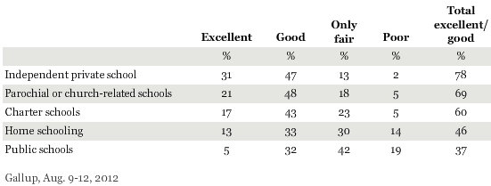 ## Practice \alert{An August 2012 Gallip poll suggests that 13\% of Americans think home schooling provides an excellent education for children. Would a random sample of 1,000 Americans where only 100 share this opinion be considered unusual?} A) No \hspace{2cm} B) **Yes** \centering{$\mu = np = 1,000 \times 0.13 = 130$} \centering{$\sigma = \sqrt{np(1-p)} = \sqrt{1,000 \times 0.13 \times 0.87} \approx 10.6$} ## Practice \alert{An August 2012 Gallip poll suggests that 13\% of Americans think home schooling provides an excellent education for children. Would a random sample of 1,000 Americans where only 100 share this opinion be considered unusual?} A) No \hspace{2cm} B) **Yes** \centering{$\mu = np = 1,000 \times 0.13 = 130$} \centering{$\sigma = \sqrt{np(1-p)} = \sqrt{1,000 \times 0.13 \times 0.87} \approx 10.6$} \raggedright Method 1: Range of usual observations: $130 \pm 2 \times 10.6 = (108.8, 151.2)$. 100 is outside this range, so would be considered unusual. ## Practice \alert{An August 2012 Gallip poll suggests that 13\% of Americans think home schooling provides an excellent education for children. Would a random sample of 1,000 Americans where only 100 share this opinion be considered unusual?} A) No \hspace{2cm} B) **Yes** \centering{$\mu = np = 1,000 \times 0.13 = 130$} \centering{$\sigma = \sqrt{np(1-p)} = \sqrt{1,000 \times 0.13 \times 0.87} \approx 10.6$} \raggedright Method 1: Range of usual observations: $130 \pm 2 \times 10.6 = (108.8, 151.2)$. 100 is outside this range, so would be considered unusual. Method 2: Z - score of observation: $Z = \frac{x-mean}{SD} = \frac{100-130}{10.6} = -2.83$. 100 is more than 2 SD below the mean, so would be considered unusual. ## Shapes of binomial distributions For this activity you will use a web applet. Go to [https://gallery.shinyapps.io/dist_calc/](https://gallery.shinyapps.io/dist_calc/) and choose Binomial coin experiment in the drop down menu on the left. - Set the number of trials to 20 and the probability of success to 0.15. Describe the shape of the distribution of number of successes. - Keeping $p$ constant at 0.15, determine the minimum sample size required to obtain a unimodal and symmetric distribution of number of successes. Please submit only one response per team. - Further considerations: - What happens to the shape of the distribution as $n$ stays constant and $p$ changes? - What happens to shape of the distribution as $p$ stays constant and $n$ changes? ## Distributions of number of successes \alert{Hollow histograms of samples from the binomial model where $p = 0.10$ and $n = 10, 30, 100, \text{and } 300.$ What happens as $n$ increases?} ```{r, echo=F, message=F, warning=F, out.width="90%",fig.align='center'} k <- -50:500 p <- 0.1 n <- c(10, 30, 100, 300) xl <- c(0, 0, 0, 10)-1 xu <- c(7, 11, 24, 50)-1 axis1 <- list() axis1[[1]] <- seq(0,6,2) axis1[[2]] <- seq(0,10, 2) axis1[[3]] <- seq(0, 20, 5) axis1[[4]] <- seq(10, 50, 10) par(mfrow=c(2,2)) for(i in 1:4){ pk <- dbinom(k, n[i], p) xlab <- paste("n =", n[i]) plot(k-0.05,pk,type='s',xlim=c(xl[i], xu[i]), axes=FALSE, xlab=xlab, ylab="", col=COL[5], lwd=2, cex.lab = 2) axis(1, axis1[[i]]) abline(h=0) } ``` ## How large is large enough? The sample size is considered large enough if the expected number of successes and failures are both at least 10. \centering{$np \geq 10$ and $n(1-p) \geq 10$} ## How large is large enough? The sample size is considered large enough if the expected number of successes and failures are both at least 10. \centering{$np \geq 10$ and $n(1-p) \geq 10$} \raggedright $10 \times 0.13 = 1.3$ and $10 \times (1-0.13) = 8.7$ ## Practice \alert{Below are four pairs of Binomial distribution parameters. Which distribution can be approximated by the bell shaped curve?} A) $n=100, p=0.95$ B) $n=25, p=0.45$ C) $n=150, p=0.05$ D) $n=500, p=0.015$ ## Practice \alert{Below are four pairs of Binomial distribution parameters. Which distribution can be approximated by the bell shaped curve?} A) $n=100, p=0.95$ B) \alert{$n=25, p=0.45 \rightarrow 25 \times 0.45 = 11.25; 25 \times 0.55 = 13.75$} C) $n=150, p=0.05$ D) $n=500, p=0.015$